3-Level Heterogeneity Model for Wireless Sensor Networks

Published Online April 2013 in MECS

The Wireless Sensor Networks (WSNs) are one of the important classes of wireless networks that have applications in several environments, e.g. in floods, volcano, battlefield surveillance, a few to name. The utility of WSNs lies in the fact that they are easily deployable, less costly, and do not require a fixed infrastructure. Most importantly, they can be used to obtain information in such environments which is not possible in any other way. More details about applications of WSNs can be found in [1,2]. Besides their variety of applications, the developments in microelectromechanical (MEM) systems based sensor technology have attracted researchers towards the WSNs. In last couple of years, different kinds of protocols have been developed as the traditional protocols are not suitable because of energy constraints in the WSNs. A wireless sensor is a tiny device consisting of four components: processing unit, sensing unit, transceiver unit, and power unit. The processing unit comprises low end processor and small amount of memory. The sensing unit contains sensing device to sense the environment (collect data) and analog to digital converter to convert the collected data into digital form for further processing. The transceiver unit connects the processing unit to external network through base station. The power unit provides the energy to all units of the sensor; however, there is not external power supply in order to provide extra energy. Besides the four units discussed above, there are application dependent units in a sensor such as location finding unit, mobilizer. A detailed survey on the wireless sensor networks can be found in [3,4]. Since the energy is the most critical constraint in a WSN, it should be used most efficiently. In other words, a network should conserve its energy for the maximum possible time without affecting the data collection in the sensing environment. The duration for which a WSN can collect data from its sensing environment is termed as its lifetime. If all sensor nodes have same amount of energy in a WSN, it is called as homogeneous WSN. There have been many studies for estimating the lifetime in a homogeneous WSN [5-11] and accordingly many protocols have been developed. These protocols can be cluster based or non-cluster based protocols. A few cluster-based protocols assume the WSNs of heterogeneous nature; while there does not seem to exist any non-cluster based protocol that assumes the WSNs of heterogeneous nature. The load balancing protocol (LBP) is an important non-cluster based protocol. It has been further improved by incorporating the adjustable sensing range and named as load balancing protocol with adjustable sensing range (ALBP). In this paper, we propose a heterogeneous model for the WSNs. This model is general enough to describe 1-level, 2-level, and 3-level heterogeneity. We also simulate ALBP protocol by using our proposed heterogeneous model and call the resultant protocol as heterogeneous ALBP (hetALBP). It is observed that the lifetime of a WSN is longer for hetALBP than the original ALBP protocol.

The rest of the paper is organized as follows. Section 2 discusses the related works. In section 3, the proposed heterogamous model for WSNs is discussed. Section 4 discusses the simulation results. Finally, the paper is concluded in section 5.

• II.    R elated W orks

There are two main classes of protocols for wireless sensor networks: cluster based and non-cluster based protocols. Some important cluster-based protocols include low energy adaptive clustering hierarchy (LEACH) protocol and its variants [12,13], stable election protocol (SEP) [14], deterministic energy efficient clustering (DEEC) protocol [15], and energy efficient hierarchical clustering (EEHC) protocol [16]. These protocols divide the sensor nodes into clusters and each cluster has its cluster head. The sensor nodes in a cluster transmit their information to the corresponding cluster head that in turn forwards that information to the base station. The non-cluster based protocols use adjusting sensing range and load balancing techniques. They include LBP [6, 7-9], deterministic energy efficient protocol (DEEPS) [8,9], ALBPS [10,11], deterministic energy efficient protocol with adjustable sensing range (ADEEPS) protocol [10,11]. Other protocols such as hybrid energy efficient distributed (HEED) protocol [17] use both the approaches that have been used in cluster based and non-cluster based protocols. We may termed them as hybrid protocols. The LEACH protocol is the very first protocol for homogeneous WSNs. It considers the predetermined number of sensor nodes as cluster heads, which are generally some percentage (e.g. 5%) of the total sensor nodes in the WSN. Later on, different variants of LEACH such as LEACH-C, LEACH-M, LEACH-V have been discussed [12,13]. The LEACH or its variants use intra-cluster communication. The HEED [17] protocol decides the cluster heads based on the probability that is given by the ratio of residual energy to the initial energy of the sensor nodes. It uses both intracluster and inter-cluster communication for homogeneous WSNs. It extends the basic scheme of the LEACH by using the residual energy as primary parameter and the network topology features (e.g. node degree, distances to neighbours) are only used as secondary parameters to break tie between candidate cluster heads, as a metric for cluster selection to achieve power balancing.

It has been observed that if the sensor nodes in a WSN are equipped with different energy levels, the WSN lifetime increases [15, 16, 18, 19]. The WSN in which the sensor nodes contain different levels of energy are called heterogeneous WSNs. Heterogeneity can be defined in terms of link, computational, and energy, but the energy heterogeneity is the most prominent as both link and computational heterogeneities depend on the energy of the network. A few works have been discussed for heterogeneous WSNs. The work [14] discusses SEP protocol by considering 2-level heterogeneity of the sensor nodes. The work [15] discusses distributed energy efficient clustering algorithm by considering 2-level and multi-level heterogeneity of the sensor nodes. The SEP and DEEC use same model for 2-level heterogeneity. For multilevel heterogeneity, the 2-level heterogeneous model has been extended by allocating different energy level to each sensor node from a prespecified energy interval. The papers [16, 19] discuss an energy efficient heterogeneous clustered scheme by considering 3-level of heterogeneity. Another work [18] discusses 3-level heterogeneity by considering the same heterogeneous model as in [16]; however, it provides longer lifetime.

In non-cluster based protocols, a sensor assumes different states such as active, idle or vulnerable /deciding state. The sensor node in active state monitors the environment and in idle state, also called sleep state, it conserves its energy. In vulnerable state, a sensor node makes decision to go to either active or sleep state. The main goal of load balancing is to keep minimum number of sensors in active state so that the network energy can be conserved to prolong lifetime. Probably the first work on load balancing is the load balancing protocol (LBP) [7]. The LBP assumes all sensor nodes to be of homogeneous nature, i.e. all nodes have same amount of energy. The DEEPS [8,9] belongs to non-cluster based class. In this protocol, a target can be sensed by two or more sensor nodes. The sensor node that has maximum effect on the target in terms of energy assumes active states and others go to their sleep state with respect to that target. Thus, only one sensor node is active for a given target. This protocol performs better than the LBP in terms of network lifetime. The LBP and DEEPS assume all sensor nodes to have fixed sensing range. The paper [5] discusses a solution of the adjustable range set covers (AR-SC) problem. In this work, the maximum number of set covers and, for each sensor in a set, a suitable sensing range is determined. The sensors in a set can cover all targets in the monitoring area. In [7-9] LBP and in [8, 9] DEEPS have been improved by incorporating adjustable sensing range. These protocols have better performance as regard to network lifetime. To the best of our knowledge, no protocol from the noncluster-based class uses the heterogeneous WSN. In this paper, we propose a heterogeneous model for the WSNs and simulate the ALBP [10,11] protocol for estimating the lifetime of a WSN. From the simulation results, it is found that the lifetime of a WSN prolongs as compared to the ALBP protocol. The main idea of ALBP is that the maximum number of sensors are kept alive as long as possible by means of load balancing (i.e., if a certain sensor is overused compared to its neighbours, then it is allowed to sleep). In ALBP, the sensors can freely change active, idle, or deciding states. In order to find the sensor cover schedule, each sensor initially broadcasts its battery level and targets covered to all neighbours and then stays in the deciding state with its maximum sensing range. When a sensor is in the deciding state with range r, it may stay in the same state or change to active or idle state. If an active sensor nearly exhausts its energy, it broadcasts this information to its neighbours. A minimal subset of neighbours in idle state will change their states into active and effectively replace the exhausted sensors. Finally, when there is a target which cannot be covered by any sensors, the network fails. In next section, we discuss our proposed heterogeneous model for wireless sensor networks.

• III.    P roposed H eterogeneity M odel

We consider a heterogeneous model of 3-level for estimating the lifetime of a wireless sensor network (WSN). Let N be the total number of sensor nodes in a WSN, which are divided into Ɵ *N, Ɵ 2*N, and Ɵ3*N number of sensor nodes in increasing order of their energy levels, where 0< Ɵ < 1. The nodes Ɵ*N may be designated as type-1 nodes, which have lowest energy level. The nodes Ɵ3*N have maximum energy and are designated as type-3 nodes. The nodes Ɵ2*N have energy that lies between type-1 and type-3 nodes and they are termed as type-2 nodes. Normalization of Ɵ, Ɵ2, and Ɵ3 gives Ɵ3 = 1- Ɵ- Ɵ2. Let E1, E2 and E3 denote the energy levels of type-1, type-2 and type-3 nodes, respectively; thus, E1 < E2 < E3. We also assume that the number of type-1 nodes is more than the number of type-2 nodes and the number of type-2 nodes is more than the type-3 nodes. This assumption is not unrealistic because the nodes having maximum energy are costliest and their number should be minimum possible in order to reduce the network cost. The nodes having least energy are cheapest and hence they can be maintained as per requirement. The total energy of the WSN, denoted by Etotal, is given by

E total =Ν∗Е ! ∗Ɵ+Ν∗Е2 ∗Ɵ2 +Ν∗Е3∗Ɵ3

It may be written as follows

Etotal =Ν∗Е! ∗Ɵ+Ν∗Е₂∗Ɵ²+Ν∗Е3 ∗ (1 - Ɵ - Ɵ²) (1)

The model given in (1) is general enough to describe 1-level (homogenous), 2-level and 3-level heterogeneity in a WSN. We first determine the range of Ɵ for which the energy E total is non-negative. This range can be obtained by solving the following equation:

Ν∗Е ∗Ɵ+Ν∗Е ∗Ɵ2 + Ν ∗Е ∗ (1 - Ɵ - Ɵ2)=0

This equation can be written as follows:

Ɵ2 *(E3-Е2 ) + Ɵ ∗ (E 3 -Е1)-Е3 = 0              (2)

Its solutions are given below:

-(E 3 -Е 1 ) -√(E 3 -Е i ) ² +4∗Е 3 ∗(E 3 -Е 2 ) 2(E3-Е2)^,

Ɵ ⁼

(E3~E1)+ √(E3~E1)2+4∗Ез ∗(E3~E2)

2(E3-E2)

The minimum and maximum values of Ɵ are given by Ɵt and Ɵ 2 , respectively. Since LB< Ɵ < 1, LB denotes lower bound of Ɵ and Eg >Et , the valid solution of (2) is Ɵ2 . Thus, we have the following (LB< Ɵ < 1)

1 ≥ ^-(E 3 -Е 1 ) + √(E 3 -Е 1 ) \ +4∗Е 3 ∗ (E 3 -Е 2 )

1 ≥                2(E 3 -Е2)

≥ LB

This can be written as follows:

2(E3 -Е2)+(E3 -Е1)≥

√(E 3-Е1)³+4∗Е3 ∗ (E 3-Е2)                     (3a)

√(E3 -Е i )2 +4∗Е3 ∗ (E3-Е2)≥2∗LB∗

(E 3-Е2)+(E3-Е1 )                          (3b)

From (4a), we have

(E 3-Е2⁾² ≥Е2 ∗ (E3-Е1)

This relation is justified as all initial energies are positive and E 3 > E 2 > E 1.

Relation (3b) helps determining LB under the given constraints.

In order to describe two types of nodes in (1), i.e., to have type-1 and type-2 nodes, we need to abolish third term in (1), which can be done by the following equation:

1-Ɵ-Ɵ2 = 0                       (4)

The solutions of (4) are (√5 - 1)/2 and (√5 + 1) / 2. Since LB< Ɵ < 1, the valid solution of (4) is Ɵ = (√5 -1)/2. For this value of Ɵ, the model in (1) contains type-1 and type-2 nodes as the third term becomes zero.

For Ɵ = 0 , we have only one type of nodes because first two terms in (1) become zero. This is the case of 1-level heterogeneity, which is also called homogeneous WSN. Here the only problem is that the model contains type-3 nodes only. This problem can be handled if we write Ɵ in terms of E 1 , E 2 , and E 3 . The simplest relation we can have is given below:

Ɵ= ^E3"^E1 ∗( e₃-e₂ )

where n is a positive integer greater than 1 (n>1). In present case, we take n=2.

The relation (5) does not assume E 1 = E 2 or E 2 = E 3 or E 1 = E 3 . It simply forces the model (1) to have type-1 nodes rather than the type-3 nodes for homogeneous case (when Ɵ = 0). It may be noted that there can be different relations of E 1 , E 2 , and E 3 for Ɵ that forces the model (1) to have type-1 nodes when it has only one type of nodes. But we have taken one of the simplest relations that forces the model (1) to have type-1 nodes, when it describes the homogenous network, in addition to satisfying all other constraints such as LB <  Ɵ <  (√5 -1)/2 and E 1 < E 2 < E 3 , where LB denotes lower bound that is determine d from (5).

When Ɵ = (√5 - 1)/2, there are two types of nodes as third term in (1) becomes zero for this value of Ɵ. In this case, the network can be considered as 2-level heterogeneous WSN. It may be noted that the model (1) contains type-1 and type-2 nodes, not type-3 nodes. F or any value of Ɵ satisfying the inequality LB≤ Ɵ ≤ (√5 -1)/2, the model contains all three types of nodes. In this case, the network can be considered as 3-level heterogeneous WSN. Thus, we have shown that the proposed energy model in (1) can describe 1-level, 2-level and 3-level heterogeneity in a WSN.

• IV.    Simulation Results

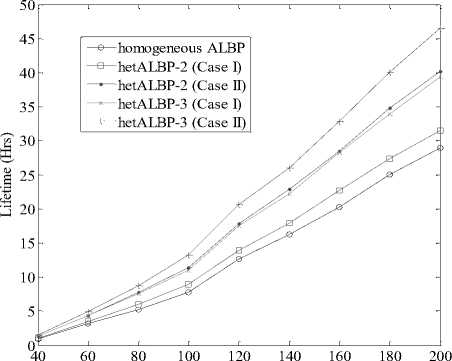
In this section, we discuss the simulation results of the ALBP protocol by using our proposed heterogeneity model; we call this implementation of ALBP as hetALBP. Our proposed model can describe 1-level, 2- level and 3- level heterogeneity of a WSN and accordingly the ALBP protocol is termed as homogeneous ALBP for 1-level heterogeneity, hetALBP-2 and hetALBP-3 for 2-level and 3-level heterogeneity, respectively. The energy models considered in our simulations are linear and quadratic, which are commonly used in literature [15]. The linear model is defined as ei = c1*ri, where c1 is constant whose value is given by c1=         and ei

( ∑r=iri)

denotes the energy needed to cover a target at distance ri. The quadratic model is defined as ei = c2*ri2 where c2, a constant, is given by c =

Etotal

It may be

( ∑r=lr? ) .

Table I: Simulation Parameters

Parameters	Symbols	Values
Number of Sensors	S	40 ~ 200
Number of Targets	T	25 & 50
Sensor initial energy	E i	2 J
Adjustable Sensing Ranges	(r 1 , r 2 )	(30m, 60m)
Communication Range	r	2* Sensing range
1- level heterogeneity Case I & Case II	E 1	2
2- level heterogeneity Case I & Case II	(E 1 ,E 2 )	(2, 2.5) & (2,4)
3- level heterogeneity	(E 1 ,E 2 ,E 3 , Ɵ)	(2, 2.5,6.5,0.56) & (2,4,14,0.60)

• A.    1-Level heterogeneity or homogeneous ALBP

For Ɵ=0, the network has nodes of single type, i.e. all nodes have same amount of energy and the network is called homogeneous network and the corresponding implementation of ALBP is termed as homogeneous ALBP protocol. As mentioned above for Ɵ=0 , our model has type-3 nodes, but by defining a suitable relation, we replace their energy by the type-1 nodes. The initial energy of a normal sensor node is taken as Е = 2J.

• B.    2-Level Heterogeneity or hetALBP-2

For Ɵ=(√5-1)⁄2 , the network model (1) consists of two types of sensor nodes only: type-1 and type-2. The type-2 nodes have more energy than the type-1 nodes and the type-1. In this case, two scenarios are considered, which are given as below:

Case I:  Еt =2,  Е2 =2.5

Case II: Е! =2, Е2 =4

To analyze the behavior of hetALBP, we should have shown simulation results for more number of cases. We indeed have carried out simulations for large number of cases and in all cases similar kind of results were obtained. Because of the repetitive nature of results, we have shown the simulation results for only two cases.

• C.    3-Level heterogeneity or hetALBP-3

When the value of Ɵ is taken such that it satisfies the inequality LB≤Ɵ≤(√5-1)/2, the network model (1) consists of three types of nodes: type-1, type-2, and type-3 nodes. The type-3 nodes have maximum energy, type-2 nodes have less energy than type-3 nodes and type-1 nodes have less energy than the type-2 nodes. In this case also, we have carried out simulations for large number of input parameters and in all cases we got similar kinds of results. Because of the repetitive nature of results, we have shown the results only for two cases, which are given below:

Case I:  Еt =2, Е2 = 2.5, Е3 = 6.5,   Ɵ=.56

Case II: Е! =2, Е2 =4,   Е3=14,   Ɵ=.60

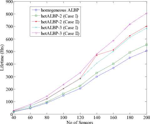
Figure. 1 Lifetime vs. Number of sensors with sensing range 30M for 25 Targets using linear energy model.

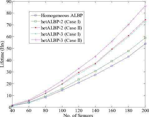
Figure. 2: Lifetime vs. Number of sensors with sensing range 30M for 25 Targets using quadratic energy model.

homogeneous ALBP hetALBP-2 (Case I)

-•-- hetALBP-2 (CaseII)

-*►-- hetALBP-3 (CaseI)

--t--hetALBP-3 (CaseII)

I 60

E 50

• ⁰40     60     80     100    120    140    160    180    200

No. of Sensors

Figure. 4: Lifetime vs. Number of sensors with sensing range 60M for 25 targets using quadratic energy model.

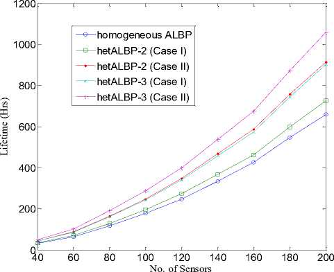
Figure. 3: Lifetime vs. Number of sensors with sensing range 60M for 25 targets using linear energy model.

homogeneous ALBP hetALBP-2 (Case I) hetALBP-2 (Case II) hetALBP-3 (Case I) hetALBP-3 (Case II)

040    60     80    100    120    140    160    180   200

No. of Sensors

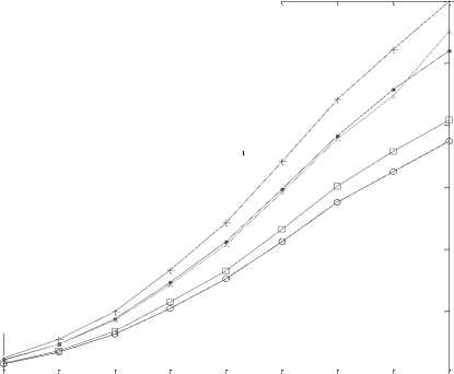
Figure. 5: Lifetime vs. Number of sensors with sensing range 30M for 50 targets using linear energy model.

No. of Sensors

Figure. 6: Lifetime vs. Number of sensors with sensing range 30M for 50 targets using quadratic energy model.

Table II: Round number when first and last nodes dead using linear and quadratic energy models in homogeneous ALBP and hetALBP for 30M sensing range, 25 targets and 200 sensors in 100x100.

Sensing range:30 M, targets:25, number of sensors:200
Cases	Linear energy model		Quadratic energy model
	First node dead	Last node dead	First node dead	Last node dead
homogeneous ALBP	492	525	36	108
hetALBP-2 (Case I)	544	575	44	116
hetALBP-2 (Case II)	688	719	60	126
hetALBP-3 (Case I)	667	705	56	120
hetALBP-3 (Case II)	795	826	70	141

Table III: Round number when first and last nodes dead using linear and quadratic energy models in homogeneous ALBP and hetALBP for 60M sensing range, 25 targets and 200 sensors in 100x100.

Sensing range:60 M, targets:25, number of sensors:200
Cases	Linear energy model		Quadratic energy model
	First node dead	Last node dead	First node dead	Last node dead
homogeneous ALBP	622	660	37	210
hetALBP-2 (Case I)	686	796	47	220
hetALBP-2 (Case II)	878	993	57	229
hetALBP-3 (Case I)	862	974	60	205
hetALBP-3 (Case II)	1018	1040	71	238

T able IV: R ound number when first and last nodes dead using linear and quadratic energy models in homogeneous ALBP and het ALBP for 30M sensing range , 50 targets and 200 sensors in 100 x 100.

Sensing range:30 M, targets:50, number of sensors:200
Cases	Linear energy model		Quadratic energy model
	First node dead	Last node dead	First node dead	Last node dead
homogeneous ALBP	358	410	16	46
hetALBP-2 (Case I)	392	449	19	50
hetALBP-2 (Case II)	505	561	28	58
hetALBP-3 (Case I)	497	552	26	53
hetALBP-3 (Case II)	585	635	31	60

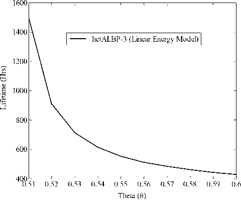
Figure. 7(a): Lifetime vs. Theta using linear energy model.

It means the network has longer lifetime in case of hetALBP protocol. Furthermore, as the level of heterogeneity increases, the number of rounds, when the first and last nodes become dead, also increases. This simply tells that the network lifetime further prolongs.

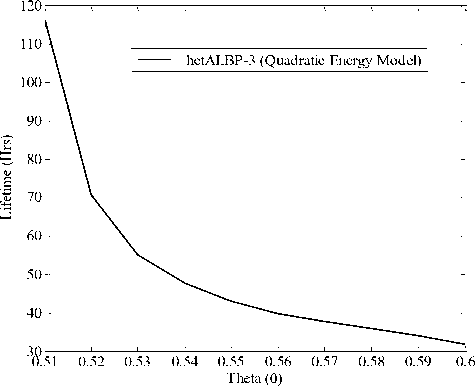
Fig. 7(b): Lifetime vs. Theta using Quadratic energy model.

Fig. 7: Lifetime vs. theta for 200 sensors with sensing range 30M and 50 targets using (a) linear energy model, (b) Quadratic energy model.

The parameter Ɵ plays very important role in our proposed heterogeneity model. Its maximum value is given by the real positive solution of (4), which should be less than 1; thus, it is upper-bounded by (√5 - 1)/2. The network lifetime for various values of Ɵ for 3-level heterogenity is shown in Figs. 7(a) and 7(b) using linear and quadratic energy models, respectively. The other input parmeters, which are fixed in our computation, are: number of sensors 200, sensing range 30m, targets 50, E1=2J and E2=2.5J. The values of E3 have been obtained from (5) for varying the value of Ɵ. We observe from these figures that as the value of Ɵ increases, the network lifetime decreases. It is logically justified because increasing the value of Ɵ increases the contribution of type-3 nodes in the network.

• V. C onclusion

In this paper, we have discussed a new heterogeneous model of 3-level for wireless sensor networks. This model is of general nature because it can describe 1-level, 2-level or 3-level heterogeneity. We have simulated the results by applying the load balancing protocol for our heterogeneous model. Our model is characterized by a parameter whose lower bound and upper bounds have been determined. Its zero value characterizes homogeneous network and its (√5 - 1)/2 value characterizes 2-level heterogeneity. For 3-level heterogeneity, its value varies from LB to (√5 - 1)/2. As the value of parameter increases, the network lifetime decreases. Furthermore, as level of heterogeneity increases, the network lifetime prolongs.