3D-reconstruction of the human brain

Author: Thaller R., Dimitrov L., Wenger E.
Journal: Компьютерная оптика @computer-optics
Section: Обработка изображений: Восстановление изображений, выявление признаков, распознавание образов
Article in issue: 9, 1991.
Free access
It is well known that the peculiar manifestations of talent are related to the morphology of human brain. The systematic researched in this field require a visualization of the individual human brain with high accuracy. This method makes it possible to accomplish a reconstruction of human brain from the series of images obtained with the use of equipment of nuclear magnetic resonance. The research of brain morphology is the basis for further visualisation of human activity through the superimposing measurements obtained by means of EEG.
Short address: https://sciup.org/14058233
IDR: 14058233
Text of the scientific article 3D-reconstruction of the human brain
This paper describes an application of image processing and computer graphics in a joint research project between the Institute of Brain Research and the Institute of Information Processing of the Austrian Academy of Sciences. The project aims at investigating the mental activities of persons with special abilities.
Our part in this project is the generation of three-dimensional representations of the human brain in computers, the calculation of two-dimensional projections of the brain from arbitrary viewpoints, and the comparison of structure and complexity of different brains. EEG-activities - measured during certain psychological tests - are mapped onto corresponding regions of the cortex.
In this paper we describe a solution for the reconstruction of the human brain starting with a sequence of NMR (Nuclear Magnetic Resonance) slices. All the slices of such a sequence are stacked, thus forming a huge data volume representing a part of the head together with the brain.
In a first preprocessing step the noise inherently present in NMR data is reduced. In a second step the segmentation of interesting regions, i.e. the outline of the brain, is done semi-automatically. We use an approximation to the well-known Marr-Hildreth operator to produce binary images. From these bilevel images brain masks are interactively selected.
At present the last step in the processing pipeline is the rendering. From all the methods proposed for displaying volume data we have chosen, ray tracing, a technique whish has been one of the major topics in computer graphics within the last few years. The problems in using the ray tracing technique in connection with the voxel representation are discussed.
Finally we show a set of pictures demonstrating the current state of the project. Future research plans include the refinement of the segmentation process and the implementation of some of the algorithms on a parallel computer architecture, namely a transputer network with a tightly coupled graohics svstem
'institute of Information Processing of the Austrian Academy of Sciences. A-1010 Vienna, Sonnenfelsgasse 19/2.
2 MOTIVATION
The motivation for this project originated from a problem in the field of human brain research, raised by Prof. Hellmuth Petsche from the Institute of Brain Research of the Austrian Academy of Sciences. It is well-known for a long time that special manifestations of talent are reflected in the morphology of the human cortex, especially in the dimension and lateral differences of certain gyri and in the complexity of the morphology of the gyri (a comprehensive review is given by Meyer [Mey77]). Until recently it was not possible to do systematical research on the morphology of human brains. The value of earlier investigations was diminished by the fact that all the available material came from either old persons with sometimes massive regressive modifications, or pathological persons.
Nowadays it is possible to visualize the morphology of the brain of healthy persons by means of nuclear magnetic resonance tomography. Without data from non-pathological brains this project would not be feasible.
Although the cortex has some common structural characteristics (e.g. the Fissura Sylvii or the central gyri), the morphology of the human brain varies from person to person and is a specific feature of each individual. This also holds true for the differences between the two hemispheres [Gal84]. Therefore it is extremely important to generate views of the individual human brain with high accuracy.
In the past years the Institute of Brain Research has proved that a specific cognitive performance of the human brain is very often correlated to changes in EEG-activity [PPR86, PRP88]. Experiments with groups of persons showed statistically significant changes of the local power density spectrum and coherence (coherence measured between adjacent electrodes and electrodes at homologous places of both hemispheres). A group of 180 persons was investigated, and all of them showed EEG-changes during the following tasks:
-
• listening to music and speech
-
• mental arithmetics
-
• reading
-
• viewing pictures and memorizing the contents of the picture
-
• verbal and visual creative thinking
Up to now the results were displayed as colored EEG probability maps on schematic maps of the cortex. This method is not satisfying, because it does not reflect the individual morphology' of the cortex. Therefore a method is presented which allows the visualization of the topography of the individual brain by calculating arbitrary shaded two-dimensional projections out of a three-dimensional representation.
-
3 MATERIALS
Within the last fifteen years two new noninvasive imaging techniques using the power and capabilities of digital computers were introduced into the radiological diagnostics, allowing the generation of high quality pictures of nearly arbitrarily oriented slices of the human body. The less recent of these techniques is the X-ray tomography, the other the nuclear magnetic resonance tomography (NMR-tomography) [Sch85, Nat86, АН84].
NMR-tomography proved to be the more appropriate imaging technique for our purpose, because it is well suited to visualize soft tissue as e.g. the brain and it allows the investigation of persons of any age and state of health without danger (as far as we know today), if there are no magnetic remnants from prior surgical intervention.
NMR-tomography uses the mutual effect between a high frequency radiation and atomic nuclei with a magnetic dipole. Among all the NMR-sensitive nuclei the hydrogen atom has an enormous importance because it is contained with a high concentration in all organic tissues. A static magnetic field (between 0.15T and 1.5T) aligns all the nuclei along that field. A high frequency radiation (between 6MHz and 60MHz) is applied in short pulses of lOOps or 500ms which changes the orientation of the nuclei from their equilibrium orientation. The nuclei return to their initial state with characteristic time constants, the so called relaxation times, thereby delivering their absorbed energy.
These relaxation times are visualized in NMR-tomograms. For further details about the physical, mathematical, and technical fundamentals we refer to the literature [RSL86, АН84].
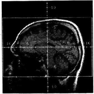
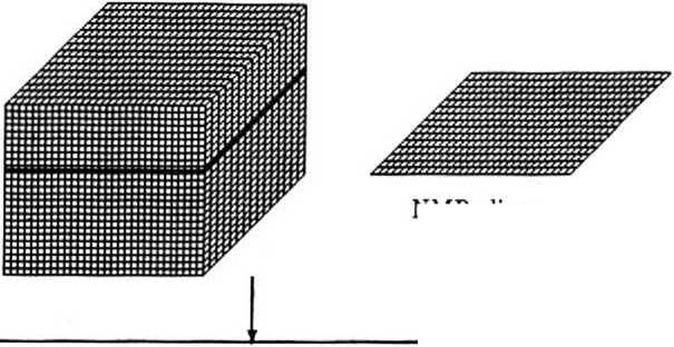
128 slices
-
Figure 1: Sagittal slice showing the scanning area.
For our project we are using NMR-images generated by a SIEMENS MAGNE-TOM with 1.5 Tesla at the Institute of Radiodiagnostic at the AKH (Allgemeines Krankenhaus) in Vienna. The resolution of one slice is 256 x 256 pixels, representing a thickness of approximately 1.2mm. 128 horizontal slices of one person are generated in about 15 minutes (Figure 1). The test person is wearing 19 dummy electrodes (of non-metallic material) fastened to the head. They are filled with the contrast medium Magnevist to mark the location of the electrodes in the NMR-images. In a subsequent EEG analysis the actual electrodes replace their dummy counterparts at identical locations.
4 PREPROCESSING
4.1 Generation of isotropic data set
4.2 Data reduction
5.1 Segmentation methods
In the preprocessing phase the data set is prepared for subsequent segmentation. This is done in three steps: scaling, data reduction, and filtering.
At the moment a typical resolution of NMR-images is 256x256 pixels. Our slices cover an area of 225mm x 225mm which yields pixels of approximately 0.88mm x 0.88mm. Since the slice thickness is about 1.2mm, the voxels of the initial data set have a spatial resolution of 0.88mm x 0.88mm x 1.2mm. The display method described below is in general not restricted to cubic voxels, but the algorithm is easier to implement and will work faster with an isotropic data volume. So the data set is first scaled in z-direction, by interpolating slices between the original ones. This can be done by using simple linear interpolation, or by using more sophisticated resampling interpolation techniques which avoid aliasing artifacts [Fan86]. As a result of this scaling, the total amount of data is slightly increased. This is a trade-off between memory requirements on one hand and speed and simplicity in the rendering phase on the other.
Available NMR-tomographs yield pixel intensities quantized with more than 8 bits (typically 12 bits). We reduce the 12 bit intensities to 8 bit intensities (because of limitations imposed by our display hardware), which is no essential loss of information. The reduction is accomplished by specifying two parameters, center and width, which map the most interesting part of the whole range of values onto a smaller range. Values between min = center - width/2 and max = center + width/2 are mapped onto the interval 0 to 255, values less than min are set to 0, values greater than max are set to 255. Besides the benefit of data reduction, the intensity value of a pixel can now be stored in one byte. This economization allows a simple data structure and fast access for the display program.
In addition the head and the brain in the images do not occupy the whole 256x256 matrix. Approximately 20% of the image is background only, which is removed for further data reduction.
of the brain with as little user interaction as possible is a very difficult task. Several different approaches have been proposed to solve this problem. All of them do need a certain amount of interactivity to specify accurately the required anatomical structures.
The most promising approaches can be divided into two categories. They either use classification models, or apply three-dimensional surface detection algorithms on the data volume.
Methods of the first category typically apply two passes. In a training phase a representative slice is chosen, and the structures (tissues) of interest are interactively segmented. Several physical and morphological features are calculated for this reference image, relevant features are determined using statistical analysis in order to calculate a pixel by pixel classifier which is approximated by a polynomial function. This training phase can be very time consuming. In the working phase the relevant features of every voxel in the volume are calculated, the classifier then yields the probability for the voxel belonging to the tissue of interest. If the degree of probability for a specific voxel is above a certain threshold, it is marked as belonging to the tissue [KL87, KL88, BSP89],
Methods of the second category use edge detection algorithms to find contours in two-dimensional images (or surfaces in three-dimensional data volumes). Various existing methods can be used to solve the problem of segmenting brain contours in NMR-images. The Marr-Hildreth operator is especially well suited for this task, because its ability to detect intensity changes at different scales is considerable, and closed contour lines are always generated. The contours can be found as zero crossings in the output of the convolution operator [BRTH87].
5.2 Marr-Hildreth operator and DOG operator
Both of the above methods are well suited for segmentation of the human brain in NMR-images. We achieved very good results with a method of the second category. In the following we give a short review of the selected method. For details see the extensive bibliography on this topic [MH80, НП83, BWH86, BRTH87, УК87].
The Marr-Hildreth operator in two dimensions is defined as the Laplacian of a Gaussian
МН^,у) = V2G(z,y)*/(z,y)
where Цх, у) is the image, G(z, y) is the two-dimensional Gaussian distribution, V2 is the Laplacian, and * is the convolution operator. The operator can be easily extended to the three-dimensional case. Unfortunately the Marr-Hildreth operation in three dimensions is very time consuming in terms of CPU-time, because the operator is not separable. However Marr and Hildreth [MH80] showed that their operator can be approximated by the difference of two Gaussians (DOG).
The following formula represents the three-dimensional DOG operator. cre and ст, are the excitatory and inhibitory space constants, and z, y, z are the spatial coordinates.
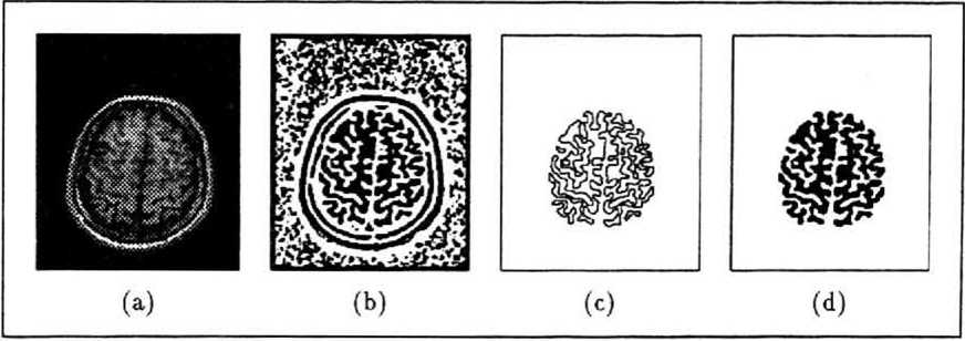
Figure 3: (a) Original slice (b) Image after applying DOG operator (c) Extracted contours (d) Brain mask
5.3 Interactive segmentation
The next step in the segmentation process has to be performed manually. Given binary images like those in Figure 3b, a user has to determine which areas constitute the brain, and select them by hand. In order to minimize the time needed for this task, a program with comfortable user interface (running on a graphics workstation) was developed. Each slice is presented to the user on the graphics display and he is requested to specify the proper areas. Selected structures are marked utilizing a floodfill algorithm which starts at a point defined by the user.
Sometimes - although rarely - wrong connections between structures remain. These bridges have to be removed interactively. When the quality of the original data set is rather poor and a lot of unwanted connections remain, we apply erosion and dilation operations to the images to remove most of the bridges.
To increase the efficiency of the interactive part of the segmentation process, results from previous slices are exploited to present a proposal for the current slice. Proceeding in a manner as described an experienced user is able to segment all the images of one data set (approximately 130 images) in about one hour. The result of this segmentation process are brain masks (Figure 3d) which can be merged with the original grey level data (Figure 3a), as will be described below. .
6 DATA REPRESENTATION
6.1 Polyhedral representation
The selection of an appropriate internal representation (data structure) is critical for the further processing steps. For the purpose of representing biological (medical) data there are two main approaches. The polyhedral representation is extensively used in traditional computer graphics for various objects, while the development of the voxel representation was demanded especially by the new medical imaging techniques. There is a lot of literature discussing the above approaches as well as alternatives. For an overview we refer to [Hoh87] and the references given there.
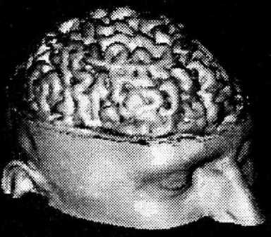
The polyhedral representation describes the surface of the objects by a set of planar polygons. This can be achieved by first examining each slice of the sequence, and extracting two-dimensional contours by using edge-finding algorithms. In a second step, the triangulation, the surface between each two consecutive slices is approximated by small triangles, trying to maximize the volume or minimize the surface, or using some heuristics [Kep75, FKU77, CS78, GD82]. The result is a polyhedral representation of the object (boundary representation). The manipulation and display of surfaces represented by polygons is well studied in computer graphics, and can be done in real time on many graphics workstations. In the past we have successfully used such methods for the display of the head (Figure 4) or inner organs such as the liver.
However, the described methods do not work well for the human brain, because all the proposed triangulation methods have problems with the high complexity and complex branching of the contours, and do not give acceptable results.
original data set
NMR-slice
PREPROCESSING generation of isotropic data set
data reduction
filtering
SEGMENTATION
convolution with DOG operator
interactive segmentation
merging brain masks with grey level data
RENDERING
specification of viewing parameters
specification of rendering parameters
shading
final image
Figure 2: Processing pipeline.
4.3 Filtering
The last step in the preprocessing of the data volume is noise reduction. Three-dimensional extensions of a median filter and linear averaging are applied to the data volume with small filter sizes such as 3x3x3 or 5x5x5 voxels. Shading takes advantage of this filtering process.
5 SEGMENTATION
6 .2 Voxel representation
The most complex task in the processing pipeline is the segmentation, i.e. the specification and extraction of interesting structures from the original NMR-slices. In the application presented here these structures are the skin (the outermost surface) and much more important, the brain (the outline of the cortex). Surfaces like the skin, which are characterized by significant changes of intensity in NMR-images, can be detected by simple thresholding, no problems are encountered. However the segmentation
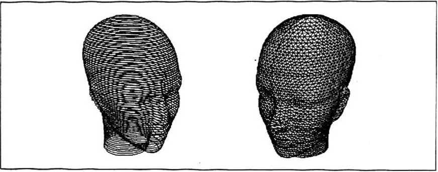
Figure 4: Wireframe of a head.
The representation we are using for our display program is simple, but expensive in terms of computer memory, compared to other representations. It is a three-dimensional array of volume elements (voxels), each voxel contains a grey level together with information from the segmentation process. In our case the whole volume consists of approximately 256x256x128 voxels, this means more than 8 megabytes of data. The disadvantage to process such a large amount of data is compensated by the applicability of sophisticated rendering algorithms, which can generate very realistic images with special effects such as transparent display of several objects. For this reason we have chosen a three-dimensional grey level volume as the basic data representation.
Having reduced the original data set as described in Section 4, the grey value of a voxel can be stored in one byte (the basic memory cell of most digital computers), which is efficient in terms of memory and access time. Since the value of the least significant bit in this byte has practically no influence on the quality of the resulting images, it is used to store other, more useful information. The output of the segmentation process (brain masks) which is one bit of information per voxel, is stored in the least significant bit. Thus we get a very comprehensive data set, containing both the grey value and the segmented brain masks in one byte per voxel.
7 RENDERING
7.1 Principles of ray tracing
7.2 Viewing
The rendering process produces shaded two-dimensional projections of the head and the brain from the three-dimensional array of volume elements. Hidden parts of the object are removed and visible parts of the object are shaded in order to create a realistic appearance. Several algorithms have been proposed to solve this problem, all of them traverse the voxels in the volume in some order. The so called back-to-front and front-to-back methods take into account the order of storage of the voxels in the computer memory, whereas the ray tracing algorithms need access to the voxels in a rather random order [FGR85, Mea82, TT84, TS87]. Since ray tracing is more flexible and powerful than the previously mentioned methods (e.g. it is easy to produce special effects such as transparency), we have implemented this method in our system.
Ray tracing has been one of the major research topics in computer graphics for several years. We will give a short introduction, and refer to the extensive literature for details [Whi80, Rog85, MT87, Gla89].
Given an arbitrary view with a projection center (eye) and a view plane (projection plane), rays are cast through every pixel of the projection plane into the data volume. The rays step through the volume and examine each voxel which they pass on their way. This process is continued until a voxel is encountered, which is found to be a surface voxel, or until the ray leaves the volume. If the ray does not find a surface voxel or even does not hit the whole volume, the corresponding pixel in the image plane is set to some background value. In the other case the corresponding pixel is set to some grey value (or color), which is calculated using a shading function.
For completely specifying an arbitrary view, the following parameters have to be supplied:
• the location of the projection center (the eye) when using perspective projection, or the direction of projection when using parallel projection,
• the projection plane (view plane),
• a coordinate system in the view plane ((u, v)-system).
• a window in the (u, v)-coordinate system.
7.3 Voxel traversal
7.4 Detection of surface voxels
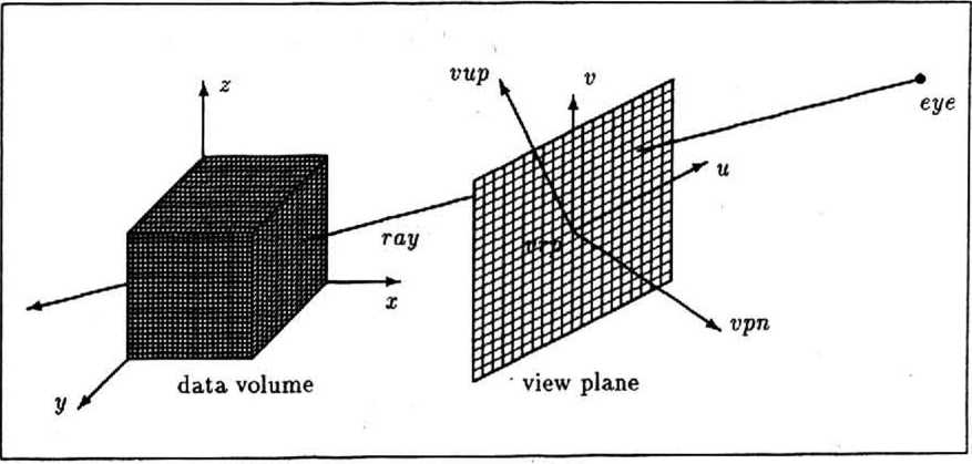
Figure 5: Viewing
The view plane is defined by its normal vector (view plane normal rpn), and a point in the plane (view reference point игр). The view reference point also serves as the origin of the (u, v)-coordinate system in the view plane. The v-coordinate axis is defined as the projection of a view up vector (vup) parallel to vpn onto the view plane. The direction of the u-axis is well-determined by the v-axis and vpn. When a window in the (u, v)-coordinate system is specified by umin, umax, vmtn, and vmai, the viewing is completely defined.
Tracing a ray’s path through the volume very fast is crucial for the performance of the display program. Generally, a ray will have to pass many voxels containing only background information, and these have to be skipped. A very efficient algorithm to accomplish this was independently developed by [CW88] and [AW87]. Cleary and Wyvill described the algorithm in much detail, with some enhancements to achieve further speed improvements. They showed, that the method can be implemented using only integer arithmetics and uses only 8 instructions in the worst case to step from voxel to voxel.
When traversing the volume, at each voxel it has to be decided whether it is a voxel on the surface of an object or not. We are interested in two different kinds of objects, the skin (defining the outermost surface of the head), and the brain.
The skin can be detected easily, because it is manifested as a significant change of intensity and thus can be found by simple thresholding. For every voxel on the ray’s path the voxel’s grey value is compared to a user defined threshold level. If the voxel’s grey value is bigger than this level the voxel represents skin.
The difficult job for the detection of the brain has already been performed by the segmentation process. During voxel traversal only the brain mask bit (see Section 6) has to be inspected.
7.5 Shading
Once a surface voxel is found, a grey value for the corresponding pixel in the image plane has to be calculated, taking into account the location of the voxel, its neighbors, some of the viewing parameters and the location of light sources which illuminate the object. For an overview of existing shading models we refer to the text books on computer graphics [FD82, Rog85, МТ87]. In the field of medical imaging the quest for realism (special optical effects) is not as emphasized as in some fields of computer graphics, resulting in the application of rather simple models. The following shading models are implemented in our system.
Distance shading: Only the distance from the observer to the point where the ray reaches the surface is taken into account. Its inverse is directly used as the grey value for the pixel in the image plane. This method is very simple, but unfortunately produces pictures of poor quality. Nevertheless it can be useful. Trying to set the viewing parameters in order to generate a specific projection can be a tedious job. In this case a number of different projections is calculated, until the desired view is produced. With the viewing parameters determined in this way, the actual image is calculated using one of the more sophisticated methods.
Lambert shading: The intensity of the pixel is calculated by the following formula, using Lambert’s cosine law, I = Lka cos 9, where 7/ is the intensity of the light source, ka is a diffuse reflection constant (0 < kd < 1) and 9 (0 < 9 < f) is the angle between the vector to the light source (L) and the surface normal (N). Using this shading function, it is possible to generate quite realistic images.
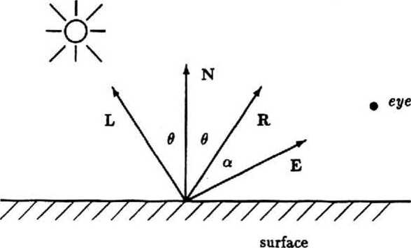
Figure 6: Shading
Phong shading: This model additionally takes into account a specular reflection component, responsible for the generation of so called highlights, as observed on shiny surfaces. We use / = Iaka + I^kdcos9 + к, cos'* a) where k, is a specular reflection constant (0 < k, < 1), and a is the angle between the direction of reflection (R) and the direction to the eye (E). The additional constant term (/a^a) is used'to simulate the effect of ambient light. Ia represents the ambient light intensity and Ла the ambient diffuse reflection constant (0 < ka < 1). Varying the power n, more or less focused highlights can be generated.
7.6 Determination of the surface normal
For shading purposes normal vectors of the surface are required. In practice the direct estimation of the normal vector from the voxel grey values gives better results than other methods, which consider only the orientation of the voxel faces [GR85, CHRU85, НВ86].
Three-dimensional grey level gradients are used as an approximation to the surface normal vector in a voxel. The gradients are calculated from the grey values of some neighborhood voxels. Given a voxel with coordinates (z, y,z) and grey value y(z,y,z), the approximated surface normal - considering the 6-connected neighborhood of the voxel (Figure 7a) - is the vector
( s(z + 1, y, z) - g(x - 1, У, z) \ 9&, у + l,z)- g(x, у - l,z) 9(x,y,z+ l)-g(x,y,z- 1) у
We have experimented with other grey level gradients computed from larger voxel neighborhoods (3x3x3 and 5x5x5 voxels), where either all or only some of the voxels in the cube (Figure 7b) contribute to the gradient calculation [HB86, TS87, ZH81]. Our investigations showed that the computational cost for inspecting neighborhoods larger than 3x3x3 voxels is not justified by the small increase of image quality.
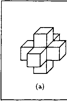
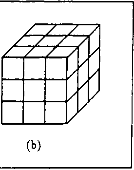
Figure 7: (a) 6-connected neighborhood (b) 3x3x3 neighborhood.
-
8 IMPLEMENTATION
The computers used for this project are
-
• Minicomputer MICRO VAX II, 11MB memory, 200MB disk, operating system ULTRIX-32 V3.0
-
• Minicomputer MICROVAX U, 9MB memory, 600MB disk, tape drive, operating system ULTRIX-32 V3.0
-
• Graphics workstation APOLLO DN3000, 4MB memory, 330MB disk, resolution 1024x800, 256 colors, operating system UNIX BSD 4.2
All three machines are integrated in a local area network (based on Ethernet and TCP/IP), permitting a fast file transfer.
The software is written in the C programming language and runs under the UNIX operating system (Berkely UNIX). All programs are written machine independent, with the exception of those portions making use of the graphics display. Very time consuming tasks such as the filtering or the segmentation with the DOG operator are done on the MICROVAX because of the large main memory available there. Programs for the interactive manipulation and segmentation of images as well as display of the calculated projections are running on the APOLLO graphics workstation and exploit the capabilities of the Graphics Primitives Resource package (GPR).
9 RESULTS
In this section we present pictures obtained from two test persons, showing the skin surface or the brain, as well as transparent display of both. The isotropic data volume consisted of 126, respectively 150 NMR-slices.
As Figures 8-9 show, grey level gradients computed from a 3x3x3 voxel neighborhood give superior (smoother) shading results than gradients derived from a 6-connected neighborhood.
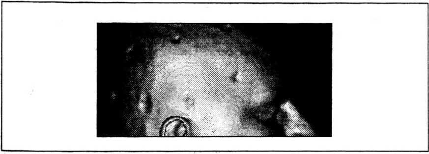
Figure 8: Grey level gradients computed from 6-connected neighborhood
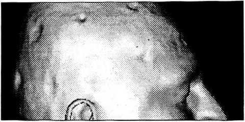
Figure 9: Grey level gradients computed from a 3x3x3 neighborhood
Figures 10-12 show the influence of different shading methods. Lambert shading is a good compromise between the rather simple distance shading and the more sophisticated phong shading with regard to image quality and processing time.
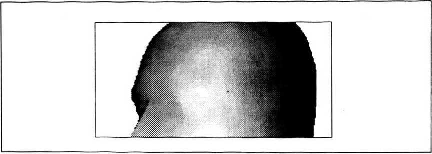
Figure 10: Distance shading
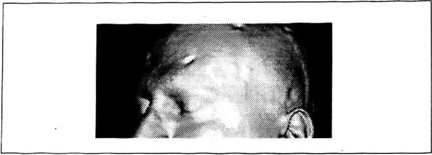
Figure 11: Lambert shading
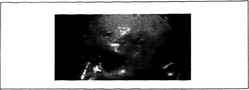
Figure 12: Phong shading
In our project the three-dimensional reconstruction of the human brain with high accuracy is of central interest. The pictures in Figures 13-17 show different views of the brain. Segmentation of the brain was performed with the DOG operator with ae = 1.1.
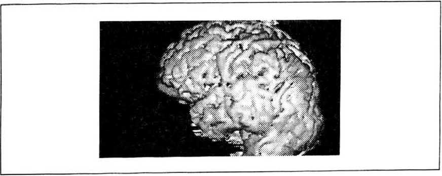
Figure 13: Left view
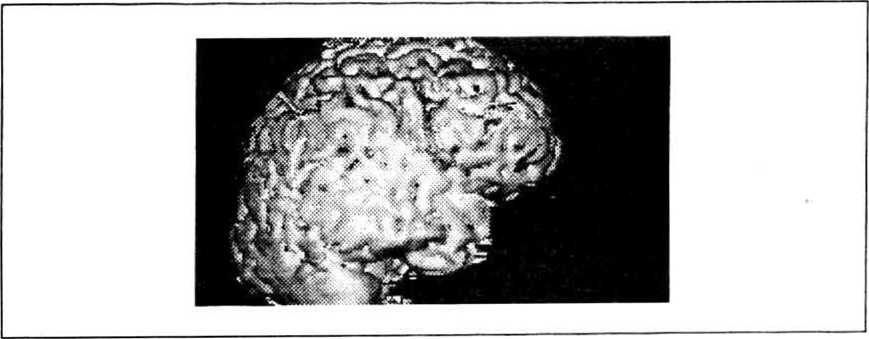
Figure 14: Right view
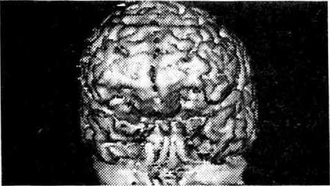
Figure 15: Front view
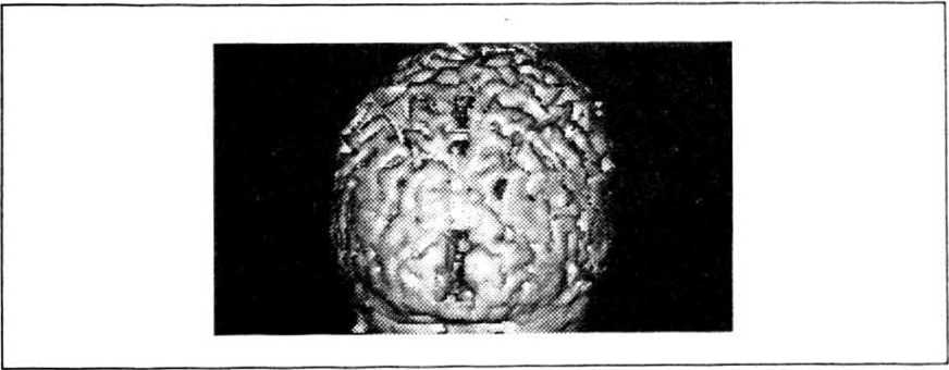
Figure 16: Rear view
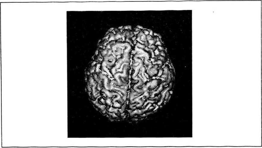
Figure 17: Top view
A combined display of the skin and the brain (Figure 18) can easily be achieved with a special option of the rendering program, which simulates transparency by forming a weighted sum of the shading values for the skin and the brain respectively: shade = a * skin + (1 — o) * brain.
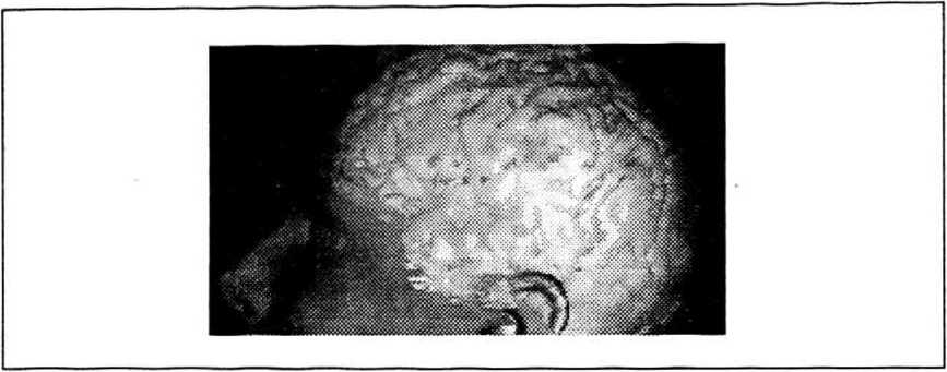
Figure 18: Transparent display of skin and brain (a = 0.7)
The last two pictures illustrate additional features of our rendering system.
-
Figure 19: Partial view of exposed cortex
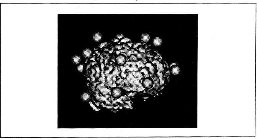
Figure 20: Display of electrode positions relative to the cortex
10 ACKNOWLEDGEMENTS
We would like to thank Prof. Petsche (Institute of Brain Research, Austrian Academy of Sciences) for initiating this project and for his encouragement and suggestions. Dr. Lindner (Institute of Brain Research, Austrian Academy of Sciences) is appreciated for many fruitfid discussions ahd assistance in the interactive segmentation. We thank Prof. Imhof and Dr. Kramer (Institute of Radiodiagnostics, AKH Vienna) for providing the NMR-data. Last but not least we are grateful to Dr. Firneis (Local Computer Center, Austrian Academy of Sciences) for useful comments and enlightening discussions.
