A Case Study in Key Measuring Software

Published Online February 2012 in MECS DOI: 10.5815/ijigsp.2012.01.01

Key duplication is a profitable business, and the service is offered today in most hardware stores. Older generations of these systems had to physically touch the original key and transmit the measures mechanically to a blade that cuts the new blank key. The blade moves along the length of the blank key and cuts the notches to the depth of the corresponding location on the original key. In these traditional devices there is no measuring system to gauge the depth and form of the notches, aside from the current location being cut. In addition, an operator must pick the correct key blank among different types of keys. By contrast, in more recent patents of key duplication systems, a measuring system is one of the most important components of the apparatus.

The newer generation of key measuring systems focuses on the innovative use of diverse light sources. Some key measuring systems use backlights to generate an image of the object’s shadows and obtain the outline of the key. Other systems employ laser technology and collimated lights to measure the depth of the key shank. Others still use uniform light sources to evenly illuminate the surface of the object. Some new developments make use of 3D cameras and high resolution cameras to capture the cuts and edges of the key as precisely as possible.

Adjusting the orientation of the key is another common problem in several kinds of key duplication systems. Without information about the position of the key in the system, it is impossible to measure the details of the key precisely enough to duplicate it. In older designs, the original key had to be attached at an appropriate location and angle, and even a slight error could lead to wrong cuts and a useless new key. Newer designs allow the system to automatically detect the position of the key, and to move it using a combination of fixation device, rotation platter and stepping motor to bring it to the correct orientation.

In this paper we introduce a new key measuring software that uses image processing techniques to achieve two main objectives: to identify the correct key blank and to find precise measures of the notches of the key shank. Given these two pieces of information, a cutting machine should be able to replicate the key. One advantage of the system we are proposing is that it eliminates the need for dedicated key measuring devices and for the use of sophisticated lighting systems and cameras. Instead, a common and commercially-available flatbed scanner is used to capture the image of the key. Furthermore, the key can be scanned with any angle and orientation; the operator no longer needs to position the key properly, nor does the system need a setup to physically move the key to the correct place. The challenge of creating sophisticated algorithms to extrapolate information from a single image and known models of the objects being analyzed is one attracting a lot of attention, and for example it has been studied in the past for the problem of face and gaze detection [1].

The rest of this paper is divided into four sections. In the next section we describe the current state of patented technology for key measurement systems as well as some relevant image processing methods. Our original image processing algorithm is detailed in section 3. The software is then thoroughly studied and tested, and the experimental results are analyzed in section 4. The concluding remarks are presented in section 5.

• II.    Review of Previous Studies

While there exists a great variety of key measuring devices, modern techniques follow a common basic principle, which consists in aiming a known light source of some kind at the key and measuring the light’s features after it hits the key using a camera. Some parts of the system, namely the key, the light source, or the camera, need to be mobile in order to measure the entire key.

Moreover, the key must often be properly oriented in the system in order to get correct measurements, which means that part of the system is dedicated to physically moving the key to the correct position. The two main types of light sources that are used in key measuring systems are laser and backlight. Laser-based systems basically work by projecting a laser line on each side of the key and measuring the deflection angle to assess the shape of the key at each point. Meanwhile, backlight systems get the outline of the key and measure the notches.

In its simplest form, a backlight-based system is one that lights the key from behind in order for the camera to get a clear shadow image of the key that serves to extract the outline of the teeth. This is the principle applied directly in [2] whereby the key is placed on a backlit transparent platform, with a camera above it. In addition, this system has a mechanism that automatically adjusts the key to its ideal position. A second light source illuminates the key from a perpendicular direction, and provided the shank of the key is not placed flatly on the transparent backlit platform, a direct light above a minimum threshold will be received by an opposite perpendicular sensor. The vertical elevation of one side of the transparent platform will be incrementally lowered until the key is positioned properly to block the perpendicular light. At this point the backlight is turned on and some pictures are taken. The number of pictures taken will obviously depend on the quality and capability of the camera used, but the system’s patent recommends that five pictures be taken. The camera is then moved in three-quarter-inch increments across a distance of about four inches and more pictures are taken at each location. These pictures are digitalized and electronically merged together to generate one silhouette of the key and its corresponding output signal. Information about the shape, depth of cut, location of cuts, and location of the shoulder, are extracted and stored in memory [2].

An alternative proposed in [3] uses both a backlight and an energized LED for more precise measurements. The light beam from the LED is projected at the key’s dents, and reflected and scattered from the surface. By keeping the projection angle constant and measuring the point of intersection of the light and the key in the image, the depth of the dents can be calculated using simple trigonometry laws. A downside of this system is that the LED light can produce glare in the images, rendering them unusable. A popular way of avoiding this problem in many other systems is to project the shadow image of the key on a screen, and have the camera measure that image instead of picturing the key itself [4], [5].

A final example of backlit systems [6] has two sources of uniform light opposite each other to generate the image of the key located between them. The sources of uniform light are capable of evenly illuminating the surface of the key without causing hot spots and glare. The first light creates a backlit image of the key that outlines its profile and notably reveals the shape of the dents. The second light then illuminates the key from the front, revealing the grooves and indentations which are used to recognise the type of key. This last system is the closest to the one we will be developing in this work. As mentioned earlier, our system uses a flatbed scanner in a way similar to the second light in [6] in the sense that it creates a frontal illumination of the key. The front-lit picture is used as the two images in [6], to get both the shape and profile of the key and information to identify its type. Our approach does create a much simpler system however. Indeed, the design of [6] duplicates the hardware and software infrastructures: it uses two different lights and two different sets of algorithms to handle the front-lit and back-lit images in order to perform a complete key measuring operation which makes the device inefficient.

A typical laser-based system, such as the one in [7], projects a laser beam at a point on the key. Collection optics in the device receive the deflected light beam onto a photo-detector, which allows the system to determine the distance to the point based on the location of the final beam on the photo-detector. The entire key is then measured point by point by moving either the laser and collection optics, or the key itself. The system in [8] uses a similar approach, but the collection optics simply detects the presence or absence of reflected light from the key, instead of the light’s position. A more sophisticated system in [9] emits the laser beam onto a series of mirrors and beam splitter, thus creating a two-beam or multi-beam setup with at least one signal beam and reference beam. The signal beam reflected from the key can be compared to the reference beam to calculate the depth of the key at that point. Once again, the entire key is measured point by point by moving part of the system. By contrast, the system in [10] is a true two-laser system. The lasers are facing each other and are symmetrical about the plane in which the key is moved. These lasers illuminate both sides of the key shank. Two video cameras are fixed relative to the lasers and are inclined relative to the planes in which light beams lie. The illuminated profile of the key is captured by the cameras and the data is then transmitted to a computer for processing [10].

• III.    Proposed Algorithm

The algorithm we propose receives as input an ordinary scanned image of a key. One of its main advantages is to eliminate the need for the complex light and laser systems described in the previous section: it simply uses an ordinary flatbed scanner, and compensates with a sophisticated algorithm to measure the shape of the key and the cuts of the key shank. This information can then be sent to a cutting device to cut the measured indentations on the extracted key blank in order to duplicate the original key, or to a 3D printer to create an entirely new key.

The pseudo-code of the algorithm we propose is shown in Figure 1. As can be seen, the first step is to convert the input image to binary format. This makes it easier to measure the positions of the cuts and different parts of the key image. Moreover, it eliminates some problems such as the local peaks in pixel intensities that are due to glare on the key image. In step 4, we cut the image into the head and shank parts of the key. Finding the correct key blank is one of the two crucial tasks of this algorithm. To this end, we need to compare those parts of the key that are the same for all keys of the same model, such as the key’s head which, unlike the shanks, remains unchanged for all keys of the same model. The moment invariants of the head are then used to model it and calculate the distances using predefined head images in a database. The closest model to the original head image found in the database provides the necessary information such as the key model name, number, and dimensions. After the system finds the correct key blank, it needs to measure the cuts and depth of dents from the shank image. It performs this task in the three steps 7 to 9 in the pseudo-code. It begins by getting the contour of the key from the image, and then refines the edge’s coordinates by interpolating the sub-pixel coordinates. It then uses the key’s dimensions, obtained previously from the database, to convert the coordinates to real-world measures. The remainder of this chapter will describe in detail each of these steps.

Input: Key Image, Key Head Database

• 1.    Binary Image ← Convert Key Image to binary format

• 2.    Binary Image ← Fill Binary Image with white pixels

• 3.    Binary Image ← Eliminate noises and gaps from Binary Image

• 4.    Head Image, Shank Image ← Cut Binary Image

• 5.    Head Image Model ← Compute geometric invariants of Head Image

• 6.    Key Model, Key Measure ← Match Head Image Model in Key Head Database

• 7.    Shank Contour Image ← Obtain the connected contour of Shank Image

• 8.    Shank Contour Image ← Sub-pixel interpolation of Shank Contour Image

• 9.    Shank Measures ← Convert the positions of Shank Contour Image into millimetres using Key Measure

Output: Key Model, Shank Measures

• Figure 1. Pseudo-code of the algorithm

• A.    The Binary Image

The first step of the algorithm is to convert the grayscale or color image taken by the scanner into a binary image. This type of conversion is already a challenge, and studies have shown that the different approach selected to do it in an algorithm’s preprocessing steps can have an impact on the quality of the final results of the algorithm [11]. In this prototype, we opted to use a simple thresholding function: the function sets all pixels with intensity greater than a threshold to white and all other pixels to black. Experimentally, we found that even a pixel with a low intensity could be an edge of the shank and must therefore be considered as part of the binary image while the scanned background is almost pure white. Moreover, simple steps such as leaving the scanner’s lid open can prevent the creation of a misleading shadow. Consequently, we set a threshold value 0.9 of the intensity of a white pixel (i.e. 230 out of 255 in a grayscale image) to detect the object. Future versions of the prototype could improve on this observation, for example by using a learning algorithm to automatically discover the optimal threshold for each given image using the 0.9 value as a starting point [12].

The resulting image, however, exhibits a lot of noise in the form of many small regions and individual pixels that are not connected to the main body of the key in the image, as well as a lot of gaps and holes inside the key. These anomalies result from darker spots in the background and lighter regions in the original scanned key, and could lead to problems later in the algorithm. To eliminate the noise pixels and the gaps and holes from the image, we invoke the fact that the key is the single largest object in the scanned picture. Consequently, we can simply retain the biggest connected component found in the image and eliminate all other regions. On the other hand, holes that are entirely surrounded by object pixels are assumed to be inside the key and are filled in. Applying these simple rules generates a single and complete image such as the one in Figure 2a. However, as can be seen in Figure 2b, irregularities remain because the filling method cannot correct gaps that are connected to the background.

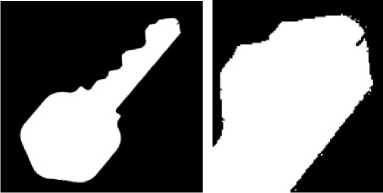
Figure 2. a: Binary image of a key. b: Irregularities visible in a closeup of a.

In order to fill in the gaps and keep the real holes inside the key head, we apply a 4-connected filter to the entire image. This filter is designed to fill in all four orthogonal neighbors of every filled pixel. Although using this method covers all the remaining gaps of the image, the resulting key image will be one pixel wider than its original size. To restore the actual size of the key, we then erode the object and remove one row of pixels on the perimeter of the key image, thus eliminating the extra layer of pixels added by the 4-connected filter.

Another drawback of this method is that it fills in the decorative holes inside the key head. These holes will be important later in the algorithm in order to compare the key with different types of key blanks. Consequently, we need to restore the holes of the key head. We start with a simple assumption: that a real hole in the key’s head will be large when compared to a gap due to an artifact of the scanning and binary conversion. Finding and restoring the largest hole in the image is simple enough, but not sufficient by itself as some keys have more than one decorative hole. Thus, after finding the biggest hole of the key, we also retrieve other holes that are close in size to that largest one and restore them as well.

When this process is completed, the binary image will be cleaned and only one connected component will remain with no gap, false holes, or irregularities.

• B.    Cutting the Image

At this stage, the two parts of the key, namely the head and the shank, will be used for two different purposes. The head of the key, being identical for all keys of the same model, will be used to recognize the key type. The shank, on the other hand, has unique cuts that must be precisely measured in order to be replicated. We use therefore the line dividing the head from the shank, which is called the joint of the key, to separate those two parts.

Telling the head from the shank would be easy, even trivial, if the key were always scanned in the same way. This would echo many existing key measuring systems, where the key must be positioned with great precision to take the measures and where even a slight deviation results in the duplicate key having the wrong cuts and being unusable. However, an important challenge in this project is to compensate for this weakness. A user of our system should be able to scan a key in any orientation, and our algorithm should automatically detect the orientation and adjust the measures accordingly. We define the orientation of the key in the image as the angle (in degrees) between the horizontal axis and the major axis of an ellipse that has the same second moments as the region [13], [14], [15]. An image moment is a function of the weighted average of the image pixels' intensities. The zeroth moment of the image is simply the area of the image:

A = ВД^ f(x,y) (1)

The centre of mass is given by the first moments:

_ S^Ey хЦх,у) _ уЦх,у) v* = ¹         "               ¹ V =         "               ¹

Sr Sy I^5C,y)        Lx Ly i^y> (2)

The second central moments are given in Equation 3:

^xx = 1x2 jXx -^i^xw)

t^v- 1цЕр6я-5>йг-№£нй9®KF = EjSp

The orientation of an object is defined as the axis of the least second moment, as given by Equation 4:

S'= ttm-¹^^- 1^+ ^((h^.- 1^)”+ 4»^_eK^aj)/ii: ti^) t/^

• > u™                                        (4)

9 = ta»^-1C 2 - ^Khm - “st +      ~ “st)²"^{1- 4} * ’W¹⁵ J?'¹ ^«m^- i^r

This gives the orientation of the major axis of an ellipse that fits the key. Next, we identify the coordinates of the top and bottom of the key. These coordinates are somewhere on the major axis line, so it is simply a matter of following that line and marking the first and last object pixels. From these two points it is straightforward to compute the coordinates of the geometric centre and the length of the key. The joint of a key is located very near the geometric centre. Specifically, we consider “very near” to be in the neighbourhood of 1/6th of the key image’s length. Taking a neighbourhood of 1/6th of the length around the geometric center, or 1/12th before the centre point to 1/12th after the centre point on the major axis, gives the cut shown in Figure 3. This figure clearly shows that there is an important change in the key’s width between the head and shank at the joint. To pinpoint the joint, we scan the neighborhood row by row, where a row has the orientation perpendicular to the major axis of the key, and for each row we count the number of object pixels. Next, we compute the difference between each two successive elements of the array. The sharpest transition we are looking for is the highest difference value between two successive rows.

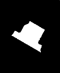
Figure 3. Image cut from 1/12th of the distance before and after the centre point of the key of Figure 2a.

A final observation is that keys are not balanced, meaning that the geometric center and the centroid are not at the same point. The head contains more of the mass of the key, and consequently the centroid will be closer to it than the geometric center. We can use this fact to figure out on which side of the joint the head is: starting from the geometric center and following the major axis, it is on the side of the joint towards the centroid.

• C.    Identifying the Key

The next stage of the algorithm is to take the image of the head cut from the original key and to match it to the correct key blank in a database. We can then retrieve the information about the key from the database, including its physical size and model number. Since we are comparing an image of the head cut from the key to other images in the database, we need to use a mathematical model of the images to make the comparison accurate and tolerant of differences in the images (such as different sizes and orientations of the heads). For this purpose, we model the images of the heads using their moment invariants, which are mathematical measures that are constant under translation, rotation, and changes in scale [16].

Given an image of size M × N, the 2D moment of order (p + q) is defined as [16] as: ,4-LS-L

mrT= ^^^^'^

х=йу=й

where p and q are integers. The corresponding central moment of order (p +q) is defined as:

Я-1Л-1

К„= ^2^Х-^Г^У-^1^У^

л=оу=»                            (6)

where я = ^ and У= Т^. The normalized central mra * mDP moment of order (p + q) is defined as:

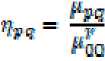
where г= + 1. The set of seven moment invariants

1          2

used in this project can be derived from the following set of equations [13]:

7i ■ to + Ure ja-te'-S'd"-^/,.)2

7a = (чт ~ Ml)” + (Ml - Чба)”

7i ■ (^30 4“ Чи)2 4- tei + Жз)2

7» = ^№ —3?fia)(wl- 4ia)|tej4- Чп^ — ?Mi + Щя^-Ь (Ml ~ И»«)(%1 + Щв)|3(»™ + 4и)2 - tel + Щи)2]

7_е - (чэд - 4(a) [ten + Пм)¹ - (чм + %?)1 + 44ii(q,-» + Чи) ( Чп + »w)

7т = (Ml ~ »№l)(»o + 41?)|(№+ ?ii)? - 3(ч»1 + Щв)1-

(>В<> - 3fB$)tei + Щи)®)?* + 4i»)2 - tei + Ям)2]-

In order to compare the seven moment invariants of two images, we simply compute the Euclidian distance between them. Since the moments can have a sign difference from one image to the next, it is necessary to take their absolute value in the following equation:

= vTET^zR7F+CT^zRn?H71U^Ey+nn44^7Q^::Qy4RJ^::l^^ (9)

Now, we can compare a head’s image to a set of images, and find the best match as the one with the smallest distance.

We created a database of key images and information, using the procedure described so far to extract the heads from the key images. Each key in the database is represented by three scans and three head images. The reason for this is that, despite the processing presented in section 3.1, differences from glare and light reflections on the key can introduce noise, and this noise can cause variations in the values of the moments invariants. Using several images of each head allows our system to average out these variations. Experimentally, we found that the average of three images was enough to deal with almost all noise problems. To further improve the noisetolerance of the system, each scanned key is used to create two head images: one that maintains the decorative holes in the head and another where those holes are filled out. By using the average of all six comparisons we greatly increase the chance of picking the correct match in the database.

Another problem that must be dealt with at this point is the fact that some keys have two joint divisions. Indeed, we find the joint of the key as the sharpest change in width in a neighborhood of 1/6th of the length of the key image around the geometric center of the key. Some keys have two such step width changes, as illustrated in figure 4. Both steps have roughly the same size, and small noise differences could make our system find either one as the joint. This width change adds or removes a bit of length from the head, which in turns causes potentially important differences in the values of the moments invariants. Our solution to this problem is to create two sets of images for keys that have two joint divisions, one set for each possible head. Both of these sets refer to the same key blank in the database.

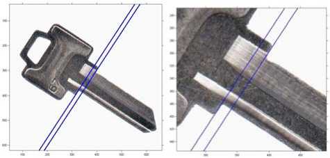
Figure 4. Left: a key with two joints. Right: close-up, showing clearly the two step changes in width.

In addition to the moment invariants, we developed a second function that works as a supplement in order to enhance the accuracy of the key blank detection. That function counts the number of pixels in head’s holes and the number of head pixels. The ratio of these two numbers is not unique for each key head image, but it can still be used as a factor to double-check and confirm our comparison results. We use this function to resolve ambiguous cases where the difference between moment invariants of two different keys is too small to guarantee that the algorithm picked the correct one.

• D.    Measuring the Cuts

The final task of the algorithm is to measure the depths of the dents of the original key. To do this, it starts with the shank side of the image extracted in section 3.2, determines an outline of the dents with sub-pixel accuracy, and then converts the coordinates into physical measures.

To identify the outline of the key, a Canny edge detector, which is a commonly-used and powerful edge detector [17] is used. This algorithm detects the details of the image clearly and produces a clean edge map, with a connected contour one pixel in thickness. But, even though each pixel in that contour represents a position along the shank of the key, measuring the positions of cuts in pixels is not accurate enough to duplicate the key. More precise sub-pixel coordinates for the points observed in the image must therefore be interpolated.

For each edge pixel detected, we will posit that the real edge lies somewhere within a 3 by 3 neighborhood centered on that pixel. Thus, for each pixel, we retrieve the intensity value of the corresponding nine-pixel neighborhood in the original grayscale key image. We further assume that this 3 by 3 neighborhood can be locally represented as a two-dimensional surface. The equation of a two-dimensional surface is a degree-two polynomial of the form given in equation (10), where x and y are the coordinates of the point, p(x,y) is the intensity of the pixel at that coordinate, and the nine ci are nine unknown constant coefficients. The nine individual pixels in the neighborhood give nine different evaluations of this equation. It thus becomes possible to solve the equation and discover unique values for the nine unknown coefficients. The Vandermonde method [18] can be applied to interpolate the equation of the surface fitting the nine points and to solve for the coefficient values. To find the edge, we must find the minimum value of this polynomial within the 3 by 3 neighborhood. Moreover, with the polynomial known, the problem becomes a simple local optimization derivation, solvable by any numerical optimization tool. The result, shown in Figure 5, is a set of sub-points around the detected edge of the key shank.

vtx.y> = с» + еуг + еду+сдху +с^х² + с₅У^г + cix^y 4- с^ху² + г»х²у² (10)

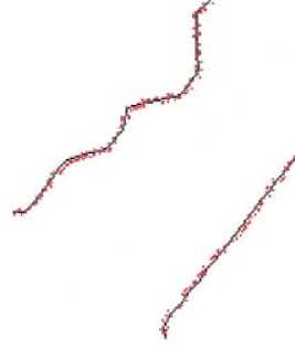
Figure 5. Sub-pixel points around the edges of a segment of the key shank. The top part of the shank has dents, while the bottom of the shank is a straight edge.

The sub-pixel points are the coordinates of the dents of the key. However, a cutting machine will need depth measures in order to cut a new key blank. These depth measures can be computed by measuring the shortest distance between each edge sub-pixel point and the major axis line of the key obtained earlier. The final challenge in this new method is to convert these depth measures from pixel values to physical measures. To do this, we need two bits of information obtained previously: specifically, the length of the key in pixels, which is simply the distance between the two ends of the key we measured in Section 3.2, and the physical size of the key, which has been retrieved from the database in Section 3.3. Comparing those two measures of the dimensions of the key gives us a conversion from pixels to millimeters, which we can then apply to convert the pixel depth measures of the dents to real-world millimeter measures.

• IV.    Experimental Results

We conducted two sets of tests to verify the two major objectives of the project, namely identifying the correct match for the original key image and measuring the depth of the cuts and edges of the original key shank.

• A.    Comparing Key Models

Section 3.3, presented a comparison of a key’s head to six images in the database, three images of the head with its decorative holes intact and three with the holes filled up. This first experiment is meant to demonstrate the need to perform this number all those of comparisons. We will now focus on 21 different scanned images of our test keys, that is three images (labeled A, B and C) for each of the 7 test keys. Figure 6 shows one image for each of the seven models for illustrative purposes. The heads of the keys were extracted using the methodology of section 3, and the seven moments invariants were computed for each head. Three keys were randomly selected as query keys that we will try to match to the correct models among the other 20. These are keys A2, A5 and A7; they should ideally be matched to keys B2 and C2, B5 and C5, and B7 and C7, respectively.

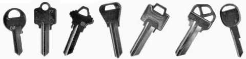
Figure 6. Test key images A1 to A7.

As explained earlier, keys are matched to those with the minimum distance in their moments invariants using equation (9). The starting point for our experiments, then, is to compute the distance between the moments invariants of the three test keys and all other keys. The results are presented in Table 1. As the table shows, when key A5 is compared to B5 and C5, the two other keys of the same type, the result corresponds to the minimum distance. However, some of the other distances are also very close to that minimum value as illustrated by the three keys of model 3. This creates the potential for confusion in the system. The test with key A2 further illustrates this problem. While B2 does give the minimal distance, three other keys, namely B5, C5 and A7, incorrectly show a smaller distance than C2. The test with A7 gives even worse results: after the correct match with B7, five heads show a smaller distance than C7. This shows that the distance between these pairs of key heads is not sufficient to pinpoint the correct match. A system that used C2 and C7 as its database head, for example, would not correctly recognize keys A2 and A7.

Table 1 ： Distance between the test keys and other head images.

	A2	A5	A7
A1	4.8909	2.4648	3.2439
B1	4.7721	2.3336	3.1203
C1	4.8349	2.3896	3.1978
A2	0	2.7090	1.7755
B2	1.1245	2.0260	1.3331
C2	1.9752	1.4203	1.1286
A3	3.5983	1.3807	2.0239
B3	3.6802	1.4175	2.1185
C3	3.7469	1.3974	2.1730
A4	4.7566	2.5368	3.1610
B4	4.3923	2.4698	2.9329
C4	4.3017	2.2962	2.7988
A5	2.7090	0	1.5842
B5	1.8914	1.3318	1.5039
C5	1.8090	1.3459	1.3229
A6	3.0202	1.7141	1.3261
B6	3.6592	2.0992	2.0975
C6	3.5032	2.1187	1.9614
A7	1.7755	1.5842	0
B7	2.4468	1.5263	1.0440
C7	2.2360	2.0892	1.5241

This first test was done using images of the keys’ heads that maintained the decorative holes. As explained in section 3, we improve accuracy by also computing the moment invariants and the distances of filled versions of key heads. To illustrate the impact of this change, the same set of comparisons of Table 1 were repeated using filled heads. The results of this second test are presented in Table 2. The table shows that errors are still present, though they are different from those in Table 1. Previously, A2 was misclassified with respect to B5, C5 and A7 in preference to C2. In the new results, those three keys exhibit a much higher distance, but C3 generates a new error. In the same vein, A7 had erroneous small distances with B2, C2, B5, C5 and A6 in Table 1. Now, four of these five keys have higher distances and only B5 remains an error, along with B6. By contrast, while the minimum distances for A5 in table 1 occurred when it was compared to keys B5 and C5, in Table 2 four errors show up with C2, B6, C6 and C7. On the other hand, the three keys of model 3, which were almost matched in Table 1, have much higher bigger distances now.

Table 2 ： Distance between the three test keys and the other head images, using filled heads.

	A2	A5	A7
A1	3.9479	5.9733	9.2432
B1	3.6977	5.7708	9.0026
C1	3.7018	5.6605	8.9675
A2	0	3.0470	5.4493
B2	1.4078	2.8008	6.1385
C2	1.9058	1.4494	4.7843
A3	2.4278	3.7288	7.2117
B3	2.1936	3.8065	7.1373
C3	1.5503	3.5142	6.5974
A4	5.1856	7.1180	10.3886
B4	5.6390	7.8020	10.9205
C4	4.6303	6.8113	9.8869
A5	3.0470	0	4.0654
B5	4.9842	2.4089	2.7318
C5	5.1465	2.4560	3.0383
A6	6.2251	3.8461	3.4573
B6	4.1904	1.5740	2.9139
C6	4.1194	1.4408	3.0365
A7	5.4493	4.0654	0
B7	6.6276	4.0183	3.0034
C7	4.5969	2.0344	2.5890

Clearly, neither the comparison between unfilled heads nor that between filled heads is sufficient by itself to pair the heads without errors. However, as noted before, the errors are mostly different between the two comparisons. Table 3 shows the results of averaging out the distance values of Tables 1 and 2. As can be seen, the low values of the correct matches in each of these tables average out to a similarly low distance value, while the erroneous matches that had a low value in one table and a high value in the other average out to a greater distance than the correct matches. Of particular interest is B5, which was an erroneous match compared to A7 in both tests. Using unfilled heads, it showed a distance of 1.5039 compared to A7, which was smaller than the 1.5241 value for C7 but bigger than the 1.0440 for B7. Using filled heads, its distance became 2.7318, which is smaller than that of B7 which stands at 3.0034 but greater than that of C7 at 2.5890. This means that B5 was always an erroneous low-distance match, but always outranked a different one of the two correct keys. After averaging out the distance values, B5 has a distance of 2.1178 with respect to A7, which is greater than the distance between A7 and B7 at 2.0237 or A7 and C7 at 2.0565.

Table 3 ： Average distance between the three test keys and the other head images.

	A2	A5	A7
A1	4.4194	4.2190	6.2435
B1	4.2349	4.0522	6.0614
C1	4.2683	4.02505	6.0826
A2	0	2.8780	3.6124
B2	1.2661	2.4134	3.7358
C2	1.9405	1.4348	2.9564
A3	3.0130	2.5547	4.6178
B3	2.9369	2.6120	4.6279
C3	2.6486	2.4558	4.3852
A4	4.9711	4.8274	6.7748
B4	5.0156	5.1359	6.9267
C4	4.4660	4.5537	6.3428
A5	2.878	0	2.8248
B5	3.4378	1.8703	2.1178
C5	3.4777	1.9009	2.1806
A6	4.6226	2.7801	2.3917
B6	3.9248	1.8366	2.5057
C6	3.8113	1.7797	2.4989
A7	3.6124	2.8248	0
B7	4.5372	2.7723	2.0237
C7	3.4164	2.0618	2.0565

Computing the average distance value of filled and unfilled versions of the same image yields the desired results for A2 and A7, but in some cases the average distance values between A5 and the two other keys of its model are not the minimum. Indeed, C2, B6 and C6 exhibit the lowest averages with respect to A5. Moreover, in some correctly-classified cases the average distance of a wrong key is not sharply greater than that of the same key type. In fact, the difference can be as low as 0.06 (or 3% of the distance value), as in the case of the A7-C7 match compared to A7-B5. Clearly the potential for errors still exists.

As explained in section 3, to further reduce the impact of noise and increase the chance of finding the correct match, we compute the distances between the original head image and three different images of a key head of each type. To this end, we computed the average distance between each test image and all three images of each type (two images for the test image’s type, since the third image is the test image). As we can see in Table 4, averaging the distance of three images gives results that are much more robust and resilient to noise. In all three sample cases, the test keys show the lowest average distance with keys of the same type. In addition, the difference between the distance of a correct and incorrect match becomes more significant. In the specific case of our previous example, the difference between A7-tpye 7 and A7-type 5 is five times higher, at 0.3 or 15% of the distance value.

Table 4 ： Average distance between the three test keys and three head images.

	A2	A5	A7
Key type No. 1	4.3075	4.0987	6.1291
Key type No. 2	2.2364	2.2420	3.4348
Key type No. 3	2.8661	2.5408	4.5436
Key type No. 4	4.8175	4.8390	6.6814
Key type No. 5	3.2645	1.8856	2.3744
Key type No. 6	4.1195	2.1321	2.4654
Key type No. 7	3.8553	2.5529	2.0401

To further illustrate the advantage of averaging out the distance results, we compared all 21 test keys with a set of one, two, and three keys. The results, shown in

Table 5, confirm that the comparison becomes more accurate when we average more sample images together. The results of Table 5 are obtained by comparing each of the 21 keys of Figure 6 with the other 20 keys. This gives a total of 420 comparisons. When using one unfilled head image only, 10 keys are matched with the wrong model. Moreover, there are 29 distances that are wrongly higher than the correct key distance, which is to say that 6.9% of distances are erroneous. Using only one filled head image gives even worse results: 11 keys are misclassified, and 38 of the distances, or 9%, are erroneous. Averaging the filled and unfilled key head images gives a small improvement in the results: 28 of the distance averages (6.7%) are erroneous and 8 out of 21 keys are not identified correctly. Although the improvement is small, it confirms that averaging both images is more accurate than using either image separately. Averaging two different key heads for each key gives better results. With three different heads per key model, there are three different pairs of key heads or 19 comparisons for each of the 21 keys and 378 average distances in total. As we can see in Table 5, the number of errors drops sharply in this case: only 3 of the 21 keys are misclassified, and only 6 of the distances, or 1.5%, are erroneous. Finally, taking the average between the original key and the three keys in each set (two keys in the set of the same key type) gives results that are nearly perfect: only one key is misclassified and only 2 distances, or 1.4% of them, are erroneous. This test illustrates the reason why we chose to have three keys of the same key type in each key set in the database.

Table 5 ： Comparison errors of all 21 keys with the database images.

Test	Count of Erroneous Distances	Count of Failed Keys
Comparing to one unfilled database head	29 errors	10 keys failed
Comparing to one filled database head	38 errors	11 keys failed
Averaging the filled and unfilled heads	28 errors	8 keys failed
Averaging two database keys (four heads)	6 errors	3 keys failed
Averaging three database keys (six heads)	2 errors	1 key failed

The only remaining errors at the end of this test occur with key type number 7 which is misclassified with key type number 5. An additional refining of the comparison is needed to deal with this problem. Looking at the images of Figure 6, we note that a clear difference between those two models is the size of the decorative hole in the key’s head. That is why we computed the ratio of hole to object pixels in Section 3.3. We can use this ratio as supplementary information to tell apart certain key models, such as 5 and 7, since, as we can see in Table 6, there is a clear difference in the ratio of those two key models. This feature however is not useful for all classifications and cannot be used as a reliable factor to identify all key types, since there are some overlaps among the ratios of other types. Indeed, while the ratios between key types number 5 and 7 have a reasonable difference, the ratio of model 7 is close to that of model 3 and the ratio of model 5 is close to that of model 4. This method could not therefore distinguish between these keys.

Table 6 ： Ratio of number of pixels in head hole to number of head’s white pixels.

	Ratio (hole pix/head pix)
A1	0.1734
B1	0.1746
C1	0.1727
A2	0.0660
B2	0.0664
C2	0.0630
A3	0.1175
B3	0.1170
C3	0.1218
A4	0.1048
B4	0.0909
C4	0.0938
A5	0.0957
B5	0.0978
C5	0.1013
A6	0.2303
B6	0.2274
C6	0.2271
A7	0.1186
B7	0.1285
C7	0.1292

The tests have so far classified the 21 sample keys compared to each other. As a final verification, we examine the classification results using the database we built as a prototype of our system. This database models the same seven models of keys and stores three pictures of each model (different from the 21 sample key pictures), plus three additional pictures for two keys that have the double-joint feature described in Section 3.3. They are key models 2 and 5. We will perform the same set of tests as before, to compare the results step by step.

We begin by computing the difference in moments invariants of the 21 test keys compared with one unfilled key head image of each key model in the database (including a second-joint picture for models 2 and 5). This generates a total of 189 difference values, of which 14 are erroneous in the sense that they correspond to wrong matches and are smaller than the values of correct matches. The error rate thus stands at 7.4%, not far from the 6.9% reported for the same test in Table 5. Note however that all these errors are confined to only two keys: B6 and C6. Next we compute the difference in moments invariants using the filled-hole version of the same database head image. This yields only 12 erroneous distances, or 6.3%, a small decrease compared to the previous test. These last results contrast with those reported in Table 5, where the filled image generated a higher error rate than the unfilled one, though the difference is minor. More importantly, the errors have changed somewhat between these two tests: six errors that occurred in the first test were corrected in the second test when the filled head was used, while four new errors appeared. All in all, four keys were misclassified, including B6 and C6. The next step now is to compute the average of the original and filled differences. Recall that in Table 5, this average led to a modest improvement of the results. In the present experiment, the results have similarly shown a slight improvement: there are again 12

erroneous differences and 4 misclassified keys, the same as with the filled head images.

The next phase of the experiment is to use a second picture of the database keys, and compute the average of four head images, using heads with and without holes for each picture. In this case, the rate of erroneous differences decreases noticeably, from 6.3% to 3.1%. This shows that the average of multiple differences is more reliable than individual differences, and confirms the results of Table 5. However, although the number of errors in the differences decreased, there are still four misclassified keys. The fact that the number of misclassified keys has not decreased is somewhat disappointing. On the other hand, it should be noted that the number of these keys has remained constant at four throughout the last tests whereas in the results reported in Table 5 their number has decreased from 11 to 3. In other words, the fixed number of four misclassified keys is close to the best result of Table 5. Furthermore, most of the errors we observe in this test are due to only one of the key types in the database, namely, type 5, which is responsible for 5 of the 6 erroneous differences. This means that we are facing a problem related to one specific key type.

The final test is to compute the average difference between the 21 keys and all three key pictures in the database. In this case, the error rate is just half what it was when only two key images were used: two keys are misclassified instead of four, and 1.5% of the differences are erroneous instead of 3.1%. This decrease in the error rate and the final values of the distances are in line with the results of Table 5. The two remaining misclassified keys both belong to model 7, and are both misclassified in model 5. This is the same misclassification that remained in Table 5. Again, by adding an extra check using the ratio of hole to object pixels in the key head, we can correct this problem.

• B.    Measuring the Dents

As explained in Section 3, once the algorithm has identified the key in the database, it measures the edges of the shank with sub-pixel accuracy. Then, by using the measure of the key known from the database, we can convert these sub-pixel coordinates into real measures that a duplicating system can use. The next set of tests examines this aspect of the system. To this end, two scanned key shanks from different models will be used. Keys B2 and B7 were randomly selected from the 21 test keys of the previous experiment, and are presented in Figure 7.

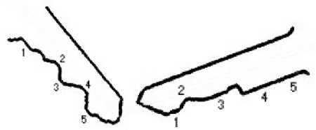
Figure 7. Two test key shanks, with five positions marked on each. Left: B2, Right: B7.

Since the main output of our system consists in measures of the shank in millimeters, the first question becomes how well these measures compare to the real dimensions of the key. To address this issue, we selected five points easy to recognize on each key, namely local maxima and minima of the dents, as shown in Figure 7. For starters, the measures of the five points were computed by the software. The real key was then measured manually using a caliper and the relative error between the real measure and the software approximation was computed using equation (11). The results are given in Table 7.

I ^pncxitSBitira— ^critg l

I TSSiUF (11)

Table 7 ： Measure (in mm) and relative error of the points marked in Figure 7.

	B2 (left)			B7 (right)
Pt	Software	Caliper	Error	Software	Caliper	Error
1	4.1	4.06	0.0099	3.2	3.30	0.0303
2	1.7	1.77	0.0395	1.7	1.77	0.0395
3	4.1	4.19	0.0214	3.0	3.04	0.0131
4	2.4	2.54	0.0551	4.3	4.31	0.0023
5	4.4	4.57	0.0372	4.1	4.31	0.0487

The average relative error of the five sample points for key B2 is 3.2%, and that for key B7 is 2.6%. These errors could be due to several factors. One factor could be the resolution of the picture: a higher-resolution scanner would provide more precise data to measure the edges. Another factor has to do with the interpolation approach: a better sub-pixel interpolation method would also yield more accurate coordinates and improve the final results.

We now turn to a verification of the consistency of the measurement of the dents. More specifically, we seek to verify how precisely the results obtained from two executions of the software using two scans of the same key will match each other. To this end, the two scans shown in Figure 8 were used and five easily-recognizable local maxima and minima on the shank were again identified for comparison purposes. Their measures and relative errors are presented in Table 8 along with caliper measures for comparison purposes.

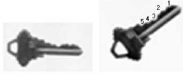
Figure 8. Two scans of the same key.

Table 8 ： Measure (in mm) and relative error of matching points on the key of Figure 8.

Pt	Software left key	Software right key	Error left to right	Caliper	Error caliper to left	Error caliper to right
1	3.7	3.6	0.028	3.30	0.121	0.091
2	4.6	4.5	0.022	4.31	0.067	0.044
3	2.1	2.0	0.048	1.90	0.105	0.052
4	3.3	3.0	0.091	3.04	0.086	0.013
5	4.4	4.1	0.068	4.31	0.021	0.049

As Table 8 shows, the average relative error between two scans of the same key is 4.4%, and in the worst case it is always below 10%. By comparison, the error between caliper measures of the original key and these images is on average 5.5%, and at most 12%. In other words, the error between two different scans of the key is a little better than the error between each scan and the real key. It thus appears that the results of the software are consistent, and not subject to variations depending on the image.

Finally, to verify the accuracy of the measurements of the dents, we compare the errors of the measures of the key calculated by our algorithm with the errors of an actual duplicate. The previous tests compared the image’s measures to those of the original key, and reported a percentage of errors. The present test will determine how these errors compare to normal key duplication errors. To conduct this test, we create a physical duplicate the key of Figure 8 using a normal hardware store’s duplication machine, and scan the original key three times to get three different sets of measures using our algorithm. We also use the same five comparison points as before. The results are presented in Table 9. As can be seen, the hardware-store key duplicate has an average relative error of 4.9%. The measures obtained by our algorithm, on the other hand, show an average error of 7.9% with the first scan, 3% with the second scan, and 1.9% with the third scan, for an overall average of 4.2% which is comparable to the physical duplicate. The results of the individual scans show that it is possible for the measures computed by the algorithm to be up to 3% better or worse than the traditional measures, which in real terms corresponds to a negligible error of a few tenths of a millimeter only.

Table 9 ： Measures (in mm) and error of a duplicate and three scans of a key.

Point	1	2	3	4	5
Original	3.30	4.31	1.90	3.04	4.31
Duplicate	3.17	4.06	1.77	2.79	4.31
Error Original to Duplicated	0.039	0.058	0.068	0.082	0.000
Scan 1	3.7	4.6	2.1	3.3	4.4
Error Original to Scan 1	0.121	0.067	0.105	0.085	0.020
Scan 2	3.5	4.4	1.9	3.2	4.4
Error Original to Scan 2	0.060	0.020	0.000	0.052	0.020
Scan 3	3.3	4.2	2.0	3.1	0.019
Error Original to Scan 3	0.000	0.025	0.052	0.019	0.002

• V.    Conclusion

This paper presents a new key measuring algorithm that is able to find the correct key blank in a key model database, and to measure the depth of the key’s dents in millimeters. This algorithm could then be connected to a cutting machine or a 3D printer to create a new copy of the original key automatically.

The main advantage of this new algorithm is that it only requires a commercially-available flatbed scanner rather than the sophisticated laser or backlight systems used today. The software uses image processing techniques to compensate the lack of accuracy in the images taken by the scanner. It also does not require the key to be adjusted to an exact position by the operator or by a physical mechanism, as many other key measuring systems do.

The development of the key model database is also an important part of this work. This database stores pictures, measures and model information about different keys. In order to find the correct match of the original key, the software compares the head of the original key with images of other key heads in the database. Using the measures retrieved from the database, the software can convert its sub-pixel coordinates of the key’s dents to actual physical depth measures.

Our results show that the algorithm can accurately find the key model in the database corresponding to a scanned key. We can minimize the effect of errors and noise by averaging the results of three database images of each model, and use some extra information such as the hole to object ratio to handle some ambiguous cases. Furthermore, the depth measures obtained by the algorithm are on par with those of a traditional hardware store’s duplicate key.

Future work should begin by extending the database. The prototype developed in this research defines seven different key models in the database. These models were selected to be a representative sample. They include both single-sided and two-sided keys, keys with double-joints, and some similar-looking key models. However, there are more than 200 key types on the market today. Covering more key types will create additional challenges, namely in the form of new ambiguous cases to handle. The comparison could also be made more accurate by using a different set of moments invariants. Indeed, Flusser and Suk [19], [20] showed that the traditional invariant set developed by Hu, which is the one used in this prototype, is missing the third order independent moment invariant. To remedy this shortcoming, they propose an extended set of moments invariants. Alternatively, Hamidi and Borji [21] propose using a set of image properties selected based on a study of biological vision and recognition to create an image recognition algorithm with improved accuracy and invariance to image distortions. It is possible that using one of these new measures will simplify the prototype by requiring fewer database images to average and will consequently reduce the number of ambiguous cases. As regards the measurement of the edges and depths of the dents of the key, our method is already comparable to those commonly used in industries today. It could nonetheless be improved by using a more accurate subpixel interpolation method.