A Classification Framework for Software Defect Prediction Using Multi-filter Feature Selection Technique and MLP

Автор: Ahmed Iqbal, Shabib Aftab

Журнал: International Journal of Modern Education and Computer Science @ijmecs

Статья в выпуске: 1 vol.12, 2020 года.

Бесплатный доступ

Production of high quality software at lower cost can be possible by detecting defect prone software modules before the testing process. With this approach, less time and resources are required to produce a high quality software as only those modules are thoroughly tested which are predicted as defective. This paper presents a classification framework which uses Multi-Filter feature selection technique and Multi-Layer Perceptron (MLP) to predict defect prone software modules. The proposed framework works in two dimensions: 1) with oversampling technique, 2) without oversampling technique. Oversampling is introduced in the framework to analyze the effect of class imbalance issue on the performance of classification techniques. The framework is implemented by using twelve cleaned NASA MDP datasets and performance is evaluated by using: F-measure, Accuracy, MCC and ROC. According to results the proposed framework with class balancing technique performed well in all of the used datasets.

Еще

Software Defect Prediction, Feature Selection, Multi-Filter Feature Selection, MLP, Artificial Neural Network, Machine Learning Techniques

Короткий адрес: https://sciup.org/15017157

IDR: 15017157 | DOI: 10.5815/ijmecs.2020.01.03

Текст научной статьи A Classification Framework for Software Defect Prediction Using Multi-filter Feature Selection Technique and MLP

Published Online February 2020 in MECS DOI: 10.5815/ijmecs.2020.01.03

Testing is one of the crucial activities in software development life cycle which aims to provide a high quality software by checking all of the developing/developed modules [33,34]. Testing is also considered as the most expensive activity which consumes more resources of the development process as compare to other activities [31,32,33]. Therefore an effective mechanism is required which can assure the high quality of end product by using limited amount of resources in testing process. Predicting the defect prone modules before the testing process is the solution of this problem. With this approach only those modules are tested which are predicted as defective. This approach can help us to deliver high quality software with limited amount of resources [5,6,18,19,20]. The process of predicting the defect prone software modules is a binary classification problem. Since last two decades, many researchers have been using the machine learning techniques to solve the problems of binary classification such as: Sentiment Analysis [7,8,9,10,11,12], Rainfall Prediction [13,14], Network Intrusion Detection [15,16], and Software Defect Prediction [1,2,3,4,5,6]. Machine learning techniques are broadly categorized in three classes: 1) Supervised, 2) Unsupervised, and 3) Hybrid [7,8,9]. Supervised technique classifies the input data into known classes. These techniques use pre-classified data (training data) to make the classification rules and then these rules are used to classify the unseen data (test data). Unsupervised techniques use specific algorithms to explore the structure of data as the classes are not known in advance. The hybrid techniques is the integration of both: supervised and unsupervised techniques. This research proposed a classification framework to detect the defect prone software modules with higher accuracy by using multi-filter feature selection technique and MLP. The proposed framework works in two dimensions 1) with oversampling technique 2) without over sampling technique. Oversampling is included in one dimension to analyze the effect of class imbalance issue [35] on classification accuracy. The framework consists of four stages: 1) Dataset Selection, 2) Data Preprocessing, 3) Classification, and 4) Reflection of Results. For implementation, twelve publically available cleaned NASA MDP datasets are used and performance is evaluated by using four accuracy measures including: F-measure, Accuracy, MCC and ROC. The results of the proposed framework with both dimensions are compared with the results of 10 widely used supervised classifiers from a published research [6]. The classifiers include: “Naïve Bayes (NB), Multi-Layer Perceptron (MLP), Radial Basis Function (RBF), Support Vector Machine (SVM), K Nearest Neighbor (KNN), kStar (K*), One Rule (OneR), PART, Decision Tree (DT), and Random Forest (RF)”. The results reflected that the proposed framework outperformed other techniques in the prediction of defect prone software modules.

II. Related Work

Machine learning techniques have been used by many researchers in order to predict the defect prone software modules. Some of the related studies are discussed here. In [1], the researcher’s proposed Hybrid Genetic algorithm based Deep Neural Network for effective software defect prediction. The purpose of Hybrid Genetic algorithm is to select the optimum features and Deep Neural Network aims to predict the modules as defective and non-defective. Datasets from PROMISE repository are used for experiments and the results reflected the higher performance of proposed technique as compared to other techniques. In [2], the researchers elaborated the importance of feature selection activity in software defect prediction process. They proposed an ANN based method for software defect prediction. They used two ANN models in the proposed technique, first they identified the optimum features by using an ANN model and then the selected features are used to predict the software defects by using another ANN model. The performance of the proposed technique was compared with Gaussian kernel SVM. For experiment, JM1 dataset is used from the NASA MDP repository. According to results, SVM performed better than ANN in binary defect classification. In [3], the researchers predicted the software bugs by using SVM. The experiment was performed by using NASA datasets including PC1, CM1, KC1 and KC3. The experimental results were compared with other techniques including Logistic Regression (LR), K-Nearest Neighbors (KNN), Decision Trees, Multilayer Perceptron (MLP), Bayesian Belief Networks (BBN), Radial Basis Function (RBF), Random Forest (RF), and Naïve Bayes, (NB). The results reflected that the performance of SVM outperformed some of the other classification techniques. In [4], the researchers predicted the software defects by using six classification techniques including: Discriminant Analysis, Principal Component Analysis (PCA), Logistic Regression (LR), Logical Classification, Holographic Networks, and Layered Neural Networks. To train ANN model, back-propagation technique was used. Performance was evaluated by using Verification Cost, Predictive Validity, Achieved Quality and Misclassification Rate. According to results, none of the used classification technique performed with 100 % accuracy. Researchers in [5] presented a framework by using feature selection and ensemble learning techniques. The proposed framework used two dimensions: with feature selection and without feature selection. Twelve publically available cleaned NASA MDP datasets are used for the implementation of the proposed framework. The performance is evaluated by using various measures including: Precision, Recall, F-measure, Accuracy, MCC and ROC. The results are compared with other well-known and widely used supervised machine learning techniques, such as: “Naïve Bayes (NB), Multi-Layer Perceptron (MLP), Radial Basis Function (RBF), Support Vector Machine (SVM), K Nearest Neighbor (KNN), kStar (K*), One Rule (OneR), PART, Decision Tree (DT), and Random Forest

(RF)”. The results showed that the proposed framework outperformed other classification techniques in some of the datasets. Researchers in [6] compared the performance of various supervised machine learning techniques on software defect prediction including: “Naïve Bayes (NB), Multi-Layer Perceptron (MLP). Radial Basis Function (RBF), Support Vector Machine (SVM), K Nearest Neighbor (KNN), kStar (K*), One Rule (OneR), PART, Decision Tree (DT), and Random Forest (RF)”. Twelve publically available cleaned NASA MDP datasets are used for this experiment and performance is evaluated in terms of Precision, Recall, F-Measure, Accuracy, MCC, and ROC Area.

III. Materials and Methods

This research presents a classification framework for the prediction of defect prone software modules by using Multi-Filter Feature Selection Technique and MultiLayer Perceptron. The framework consists of four stages: 1) Dataset Selection, 2) Data Pre Processing 3) Classification and 4) Reflection of Results.

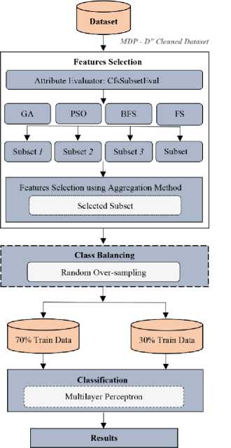
Fig. 1. Proposed Framework

The proposed framework is implemented in WEKA, which is a widely used data mining tool, developed in Java language at the University of Waikato, New Zealand. First stage of the proposed framework is the selection of relevant dataset. We have implemented the framework on twelve publically available cleaned NASA MDP datasets. The datasets include: “CM1, JM1, KC1, KC3, MC1, MC2, MW1, PC1, PC2, PC3, PC4 and PC5 (Table 1)”.

Each of the used dataset represents a particular software system of NASA and consists of various attributes/features along with the known output class (target class). The target/output class is the dependent attribute and the remaining attributes are known as independent attributes. The dependent attribute is predicted on the basis of independent attributes. The independent attributes are the quality metrics of software systems. The target class in the used datasets has either one of the following values: “Y” or “N”. “Y” means that the particular instance (module) is defective and “N” means it is non-defective. The researchers in [21] provided two versions of clean NASA MDP datasets: DS’ (“which included duplicate and inconsistent instances”) and D’’ (“which do not include duplicate and inconsistent instances”). We have used D’’ (Table 1) version in this research which is taken from [22]. These cleaned datasets are already used and discussed by [5,6], [23,24,25], [35].

Table 1. Nasa Cleaned Datasets D’’ [21]

Dataset	Attributes	Modules	Defective	NonDefective	Defective (%)
CM1	38	327	42	285	12.8
JM1	22	7,720	1,612	6,108	20.8
KC1	22	1,162	294	868	25.3
KC3	40	194	36	158	18.5
MC1	39	1952	36	1916	1.8
MC2	40	124	44	80	35.4
MW1	38	250	25	225	10
PC1	38	679	55	624	8.1
PC2	37	722	16	706	2.2
PC3	38	1,053	130	923	12.3
PC4	38	1,270	176	1094	13.8
PC5	39	1694	458	1236	27.0

Data Preprocessing is the second stage of proposed framework which consists of feature selection and class balancing activities. The proposed framework works in two dimensions, in first dimension, the preprocessing stage only consists of feature selection activity. However, in second dimension, along with feature selection activity, a class balancing technique is also included. The class balancing technique can help us to analyze the effects of imbalanced datasets on the performance of proposed classification framework. Feature selection activity aims to select the optimum set of features so that the classification results with higher accuracy can be achieved. It has been reported by many researchers that in most of the datasets only few of the independent features can predict the target class effectively and remaining features don’t only participate but can reduce the performance of classification model, if not removed. In this research, we have incorporated an aggregation based multi-filter feature selection technique, in which CFS [28,29,30] is used as attribute evaluator along with four widely used search methods including: GA, PSO, BFS, and FS. For each of the used dataset, feature selection is performed with all of these four search methods. In this process, if any particular feature is selected with any search method then 1 score is given to that feature and same process is repeated with second search method and so on. After implementing all search methods, scores of each feature in all the search methods are aggregated and only those features are selected which have at least 1 aggregated score (which feature is selected by at least one search method) as shown in Fig 2. This process is repeated for all of the used datasets.

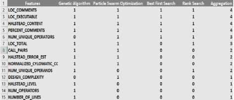
Fig. 2. Multi-Filter Feature Selection Aggregation Method

Class Balancing is the optional activity of preprocessing stage which aims to resolve the issue of “Imbalance ratio” [26,27], [35] in datasets. We have used Random Over Sampling (ROS), which reduces the imbalance ratio in dataset by duplicating the instances in minority class. This approach increases the volume of dataset due to duplication. Classification is the third stage in which we have used Feed-Forward Artificial Neural Network (Multi-Layer Perceptron). MLP contains at-least three layers: an input layer, one hidden layer and an output layer (hidden layers can be increased). It follows a supervised learning technique known as Back-Propagation for training. We have tuned the ANN (Table 2) with hit and trail approach.

Table 2. MLP Configuration

Parameter	Value
Hidden Layers	2
Number of Neurons	10
Learning Rate	0.1
momentum	0.3

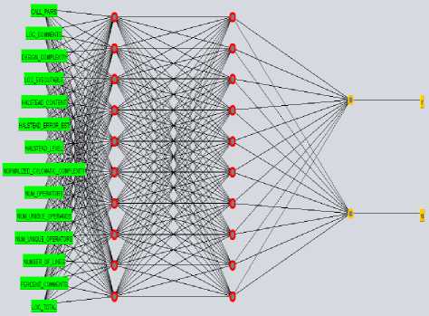
Fig 3. Multi-Layer Perceptron Architecture

Fig. 3 shows the structure of developed ANN model. First layer (From left) is the input layer which consists of the independent features of the dataset, followed by the 2 hidden layers and finally the output layer which shows either the particular module (instance is defective or non- defective). Fourth stage deals with the reflection of results. In results we have only focused on the defective class which means that the scores are only extracted and compared for the prediction of defective modules. Results are discussed in detail in the next section.

Precision * Recall * 2

F-measure =-----—-----------

(Precision + Recall)

Accuracy is the ratio of correctly classified instances to all instances

IV. Results and Discussion

This section evaluates the performance of proposed framework. The accuracy measures used for the evaluation include: F-measure, Accuracy, MCC and ROC. All these measures are generated from the parameters of confusion matrix (Fig. 4) [5,6], [35].

Accuracy =

TP + TN

TP + TN + FP + FN

AUC measures that how well a parameter can distinguish between two classes (defective/non-defective)

AUC =

1 + TP_r - FP_r

MCC reflect the ratio of the observed classifications to the predicted classification.

Actual Values

Defective (Y) Non-defective (N)

Defective (Y)	TP	FP
Non-defective (N)	FN	TN

Fig 4. Confusion Matrix

MCC =

________ TN * TP - FN * FP ________ 4 ( FP + TP )( FN + TP )( TN + FP )( TN + FN )

The parameters used in the confusion matrix are discussed below [5,6], [35]:

True Positive (TP): “Instances which are actually positive and also classified as positive”.

False Positive (FP): “Instances which are actually negative but classified as positive”.

False Negative (FN): “Instances which are actually positive but classified as negative”.

True Negative (TN): “Instances which are actually negative and also classified as negative”.

The calculation formula and brief description of all of the used performance measures are given below:

To calculate the F-measure, we have to calculate Precision and Recall first as the F-measure is the average of both of these metrics.

Precision is the ratio of True Positive (TP) instances with respect to total number of instances, which are classified as positive.

The results of both the dimensions of proposed framework are compared with the published results of 10 widely used classifiers from the paper [6]. The published paper used the same datasets (NASA MDP D’’) and performance measures for performance evaluation. The classifiers used in the published paper [6] are “Naïve Bayes (NB), Multi-Layer Perceptron (MLP). Radial Basis Function (RBF), Support Vector Machine (SVM), K Nearest Neighbor (KNN), kStar (K*), One Rule (OneR), PART, Decision Tree (DT), and Random Forest (RF)”. The results of the proposed framework along with the results of other classifiers from [6] in terms of F-Measure, Accuracy, ROC and MCC for Y class are reflected in the tables (from Table 3 to Table 14). Highest scores in each class are highlighted in bold for easy identification. The symbol ‘?’ in the results indicates that the score of the performance measure in the particular technique cannot be calculated due to class imbalance issue [6].

Precision =--------- ( TP + FP )

Recall is the ratio of True Positive (TP) instances with respect to total number of instances, which are actually positive.

Re call =

( TP + FN )

Table 3. CM1 Results

Classifier	F-Measure	Accuracy	ROC Area	MCC
NB	0.190	82.653	0.703	0.097
RBF	?	90.816	0.702	?
SVM	?	90.816	0.500	?
kNN	0.083	77.551	0.477	-0.037
kStar	0.083	77.551	0.538	-0.037
OneR	0.000	85.714	0.472	-0.074
PART	?	90.816	0.610	?
DT	0.154	77.551	0.378	0.041
RF	00.000	89.795	0.761	-0.032
MLP	00.000	86.734	0.634	-0.066
MLP-FS	0.000	89.795	0.777	-0.032
MLP-FS-ROS	0.800	79.591	0.813	0.592

Results of CM1 dataset are reflected in Table 3. It can be seen that MLP-FS-ROS performed better in F-Measure, ROC Area and MCC whereas in Accuracy, RBF, SVM, and PART outperformed others.

Table 4. JM1 Results

Classifier	F-Measure	Accuracy	ROC Area	MCC
NB	0.318	79.835	0.663	0.251
RBF	0.181	80.397	0.713	0.215
SVM	?	79.188	0.500	?
kNN	0.348	73.963	0.591	0.186
kStar	0.355	75.993	0.572	0.212
OneR	0.216	77.158	0.543	0.126
PART	0.037	79.490	0.714	0.104
DT	0.348	79.101	0.671	0.252
RF	0.284	80.181	0.738	0.244
MLP	0.146	80.354	0.702	0.206
MLP-FS	0.175	80.44	0.712	0.216
MLP-FS-ROS	0.558	62.78	0.682	0.275

Results of JM1 dataset are shown in Table 4. MLP-FS-ROS performed better in F-Measure and MCC whereas MLP-FS performed better in Accuracy and RF performed better in ROC Area.

Table 5. KC1 Results

Classifier	F-Measure	Accuracy	ROC Area	MCC
NB	0.400	74.212	0.694	0.250
RBF	0.362	78.796	0.713	0.347
SVM	0.085	75.358	0.521	0.151
kNN	0.395	69.341	0.595	0.190
kStar	0.419	72.206	0.651	0.238
OneR	0.256	73.352	0.551	0.147
PART	0.255	76.504	0.636	0.239
DT	0.430	75.644	0.606	0.291
RF	0.454	77.937	0.751	0.346
MLP	0.358	77.363	0.736	0.296
MLP-FS	0.435	77.6504	0.729	0.331
MLP-FS-ROS	0.641	62.7507	0.703	0.256

Table 5 reflects the results of KC1 dataset. It can be seen that MLP-FS-ROS performed better in F-Measure. RBF performed better in Accuracy and RF performed better in ROC Area and MCC.

Table 6. KC3 Results

Classifier	F-Measure	Accuracy	ROC Area	MCC
NB	0.421	81.034	0.769	0.309
RBF	0.000	77.586	0.735	-0.107
SVM	?	82.758	0.500	?
kNN	0.364	75.862	0.617	0.218
kStar	0.300	75.862	0.528	0.154
OneR	0.375	82.758	0.619	0.295
PART	0.143	79.310	0.788	0.056
DT	0.300	75.862	0.570	0.154
RF	0.235	77.586	0.807	0.111
MLP	0.375	82.758	0.733	0.295
MLP-FS	0.286	82.758	0.723	0.236
MLP-FS-ROS	0.588	63.793	0.730	0.358

Results of KC3 datasets are shown in Table 6. It shows that MLP-FS-ROS performed better in F-Measure and MCC whereas SVM, OneR, MLP, and MLP-FS performed better in Accuracy. In ROC Area, RF outperformed all other techniques.

Table 7. MC1 Results

Classifier	F-Measure	Accuracy	ROC Area	MCC
NB	0.217	93.856	0.826	0.208
RBF	?	97.610	0.781	?
SVM	?	97.610	0.500	?
kNN	0.333	97.269	0.638	0.325
kStar	0.182	96.928	0.631	0.174
OneR	0.200	97.269	0.568	0.206
PART	0.333	97.269	0.684	0.325
DT	?	97.610	0.500	?
RF	0.000	97.440	0.864	-0.006
MLP	?	97.610	0.805	?
MLP-FS	?	97.610	0.796	?
MLP-FS-ROS	0.853	83.105	0.900	0.680

MC1 results are shown in Table 7. It can be seen that MLP-FS-ROS showed better performance in F-Measure, ROC Area and MCC whereas RBF, SVM, DT, MLP, and MLP-FS performed better in Accuracy.

Table 8. MC2 Results

Classifier	F-Measure	Accuracy	ROC Area	MCC
NB	0.526	75.675	0.795	0.444
RBF	0.444	72.973	0.766	0.371
SVM	0.222	62.162	0.514	0.040
kNN	0.545	72.973	0.668	0.374
kStar	0.348	59.459	0.510	0.062
OneR	0.316	64.864	0.553	0.137
PART	0.667	78.378	0.724	0.512
DT	0.435	64.864	0.615	0.189
RF	0.48	64.864	0.646	0.216
MLP	0.519	64.864	0.753	0.243
MLP-FS	0.364	62.162	0.686	0.111
MLP-FS-ROS	0.667	75.675	0.694	0.538

Results of MC2 datasets are reflected in Table 8. It shows that MLP-FS-ROS performed better in F measure and MCC whereas PART performed better in Accuracy and NB performed better in ROC Area.

Table 9. MW1 Results

Classifier	F-Measure	Accuracy	ROC Area	MCC
NB	0.435	82.666	0.791	0.367
RBF	?	89.333	0.808	?
SVM	?	89.333	0.500	?
kNN	0.444	86.666	0.705	0.373
kStar	0.133	82.666	0.543	0.038
OneR	0.200	89.333	0.555	0.211
PART	0.167	86.666	0.314	0.110
DT	0.167	86.666	0.314	0.110
RF	0.182	88.000	0.766	0.150
MLP	0.632	90.666	0.843	0.589
MLP-FS	0.400	92.000	0.845	0.479
MLP-FS-ROS	0.790	77.333	0.865	0.544

Table 9 shows that in MW1 dataset MLP-FS-ROS performed better in F-Measure, ROC Area, and MCC whereas MLP-FS performance better in Accuracy.

Table 10. PC1 Results

Classifier	F-Measure	Accuracy	ROC Area	MCC
NB	0.400	89.705	0.879	0.400
RBF	0.154	94.607	0.875	0.161
SVM	?	95.098	0.500	?
kNN	0.286	92.647	0.629	0.247
kStar	0.176	86.274	0.673	0.128
OneR	0.154	94.607	0.545	0.161
PART	0.462	93.137	0.889	0.440
DT	0.500	93.137	0.718	0.490
RF	0.429	96.078	0.858	0.459
MLP	0.462	96.568	0.779	0.538
MLP-FS	0.429	96.078	0.903	0.459
MLP-FS-ROS	0.900	89.655	0.955	0.793

Table 13. PC4 Results

Classifier	F-Measure	Accuracy	ROC Area	MCC
NB	0.404	86.089	0.807	0.334
RBF	0.250	87.401	0.862	0.279
SVM	0.286	88.189	0.583	0.342
kNN	0.438	85.826	0.667	0.359
kStar	0.330	81.889	0.734	0.225
OneR	0.361	87.926	0.614	0.352
PART	0.481	85.301	0.776	0.396
DT	0.583	86.876	0.834	0.514
RF	0.532	90.288	0.945	0.516
MLP	0.562	89.763	0.898	0.515
MLP-FS	0.447	88.976	0.891	0.432
MLP-FS-ROS	0.847	84.776	0.925	0.700

PC1 results are shown in Table 10. It can be seen that MLP-FS-ROS performed better in F-Measure, ROC Area, and MCC whereas MLP performed better in Accuracy.

PC4 results are shown in Table 13. It is shown that MLP-FS-ROS performed better in F-Measure, and MCC whereas RF performed better in Accuracy and ROC Area.

Table 11. PC2 Results

Classifier	F-Measure	Accuracy	ROC Area	MCC
NB	0.000	94.470	0.751	-0.028
RBF	?	97.695	0.724	?
SVM	?	97.695	0.500	?
kNN	0.000	96.774	0.495	-0.015
kStar	0.167	95.391	0.791	0.146
OneR	0.000	97.235	0.498	-0.01
PART	0.000	96.774	0.623	-0.015
DT	?	97.695	0.579	?
RF	?	97.695	0.731	?
MLP	0.000	96.774	0.746	-0.015
MLP-FS	?	97.695	0.748	?
MLP-FS-ROS	0.918	91.244	0.920	0.838

Table 14. PC5 Results

Classifier	F-Measure	Accuracy	ROC Area	MCC
NB	0.269	75.393	0.725	0.245
RBF	0.235	75.590	0.732	0.251
SVM	0.097	74.212	0.524	0.173
kNN	0.498	73.031	0.657	0.314
kStar	0.431	69.881	0.629	0.227
OneR	0.387	71.259	0.594	0.209
PART	0.335	75.787	0.739	0.274
DT	0.531	75.000	0.703	0.361
RF	0.450	75.984	0.805	0.322
MLP	0.299	74.212	0.751	0.216
MLP-FS	0.247	74.803	0.727	0.218
MLP-FS-ROS	0.734	70.866	0.779	0.420

Table 11 reflects the results of PC2 dataset. It shows that MLP-FS-ROS performed better in F-Measure, ROC Area, and MCC whereas RBF, SVM, DT, RF, MLP-FS performed better in Accuracy.

Table 12. PC3 Results

Classifier	F-Measure	Accuracy	ROC Area	MCC
NB	0.257	28.797	0.773	0.088
RBF	?	86.392	0.795	?
SVM	?	86.392	0.5	?
kNN	0.353	86.075	0.616	0.294
kStar	0.267	82.594	0.749	0.173
OneR	0.226	87.025	0.562	0.245
PART	?	86.392	0.79	?
DT	0.358	86.392	0.664	0.304
RF	0.226	87.025	0.855	0.245
MLP	0.261	83.86	0.796	0.183
MLP-FS	0.145	85.126	0.828	0.114
MLP-FS-ROS	0.787	75.949	0.836	0.545

Results of PC3 datasets are shown in Table 12. It can be seen that MLP-FS-ROS performed better in F-Measure, and MCC whereas OneR and RF performed better in Accuracy and RF performed better in ROC Area.

Table 14 reflects the results of PC5 dataset. It can be seen that MLP-FS-ROS performed better in F-Measure, and MCC whereas RF performed better in Accuracy and ROC Area.

The results reflect the good performance of the proposed framework especially with class balancing (ROS) dimension. It has been observed that the proposed framework with class balancing technique performed better in at-least one and maximum in three performance measures on every dataset. Moreover, it has also been observed that the dimension with class balancing technique (mlp-fs-ros) did not perform well in Accuracy measure on any of the used dataset. As in most of the datasets the Accuracy is improved with the dimension where class balancing technique is not used (MLP-FS), so, this issues should be further investigated that either the ROS technique is the reason of the lower performance in Accuracy or it is something else. The proposed framework with ROS technique has fully resolved the class balancing issue [35].

V. Conclusion

This research presented multi-filter feature selection based classification framework for software defect prediction. For defect prediction, the framework uses Artificial Neural Network (MLP). The oversampling technique is also used in the framework to analyze the effect of class imbalance issue on classification performance. For experiment, 12 publically available NASA MDPI cleaned datasets are used including: “CM1, JM1, KC1, KC3, MC1, MC2, MW1, PC1, PC2, PC3, PC4 and PC5. The performance of the proposed framework is compared with 10 well known supervised classification techniques including: “Naïve Bayes (NB), Multi-Layer Perceptron (MLP), Radial Basis Function (RBF), Support Vector Machine (SVM), K Nearest Neighbor (KNN), kStar (K*), One Rule (OneR), PART, Decision Tree (DT), and Random Forest (RF)”. From the analysis of results, it has been observed that the proposed framework with oversampling technique performed well than other classifiers in F-measure, ROC and MCC measures however the Accuracy measure is not significantly improved. This issue should be further investigated that why class balancing technique has degraded the accuracy while other measures were significantly improved in most of the datasets. It has already been reported in our previously published research that Accuracy and ROC both are not sensitive to class imbalance issue in dataset (these measure don’t react either data has class imbalance issue or not). It is also suggested for future work that an ensemble of classifiers should be included in the proposed framework to further improve the performance.

Список литературы A Classification Framework for Software Defect Prediction Using Multi-filter Feature Selection Technique and MLP

C. Manjula and L. Florence, “Deep neural network based hybrid approach for software defect prediction using software metrics,” Cluster Comput., pp. 1–17, 2018.
I. Gondra, “Applying machine learning to software fault-proneness prediction,” J. Syst. Softw., vol. 81, no. 2, pp. 186–195, 2008.
K. O. Elish and M. O. Elish, “Predicting defect-prone software modules using support vector machines,” J. Syst. Softw., vol. 81, no. 5, pp. 649–660, 2008.
F. Lanubile, A. Lonigro, and G. Visaggio, “Comparing Models for Identifying Fault-Prone Software Components,” Proc. Seventh Int’l Conf. Software Eng. and Knowledge Eng., pp. 312–319, June 1995.
A. Iqbal, S. Aftab, I. Ullah, M. S. Bashir, and M. A. Saeed, “A Feature Selection based Ensemble Classification Framework for Software Defect Prediction,” Int. J. Mod. Educ. Comput. Sci., vol. 11, no. 9, pp. 54-64, 2019.
A. Iqbal, S. Aftab, U. Ali, Z. Nawaz, L. Sana, M. Ahmad, and A. Husen “Performance Analysis of Machine Learning Techniques on Software Defect Prediction using NASA Datasets,” Int. J. Adv. Comput. Sci. Appl., vol. 10, no. 5, 2019.
M. Ahmad, S. Aftab, I. Ali, and N. Hameed, “Hybrid Tools and Techniques for Sentiment Analysis: A Review,” Int. J. Multidiscip. Sci. Eng., vol. 8, no. 3, 2017.
M. Ahmad, S. Aftab, S. S. Muhammad, and S. Ahmad, “Machine Learning Techniques for Sentiment Analysis: A Review,” Int. J. Multidiscip. Sci. Eng., vol. 8, no. 3, p. 27, 2017.
M. Ahmad and S. Aftab, “Analyzing the Performance of SVM for Polarity Detection with Different Datasets,” Int. J. Mod. Educ. Comput. Sci., vol. 9, no. 10, pp. 29–36, 2017.
M. Ahmad, S. Aftab, and I. Ali, “Sentiment Analysis of Tweets using SVM,” Int. J. Comput. Appl., vol. 177, no. 5, pp. 25–29, 2017.
M. Ahmad, S. Aftab, M. S. Bashir, and N. Hameed, “Sentiment Analysis using SVM: A Systematic Literature Review,” Int. J. Adv. Comput. Sci. Appl., vol. 9, no. 2, 2018.
M. Ahmad, S. Aftab, M. S. Bashir, N. Hameed, I. Ali, and Z. Nawaz, “SVM Optimization for Sentiment Analysis,” Int. J. Adv. Comput. Sci. Appl., vol. 9, no. 4, 2018.
S. Aftab, M. Ahmad, N. Hameed, M. S. Bashir, I. Ali, and Z. Nawaz, “Rainfall Prediction in Lahore City using Data Mining Techniques,” Int. J. Adv. Comput. Sci. Appl., vol. 9, no. 4, 2018.
S. Aftab, M. Ahmad, N. Hameed, M. S. Bashir, I. Ali, and Z. Nawaz, “Rainfall Prediction using Data Mining Techniques: A Systematic Literature Review,” Int. J. Adv. Comput. Sci. Appl., vol. 9, no. 5, 2018.
A. Iqbal and S. Aftab, “A Feed-Forward and Pattern Recognition ANN Model for Network Intrusion Detection,” Int. J. Comput. Netw. Inf. Secur., vol. 11, no. 4, pp. 19–25, 2019.
A. Iqbal, S. Aftab, I. Ullah, M. A. Saeed, and A. Husen, “A Classification Framework to Detect DoS Attacks,” Int. J. Comput. Netw. Inf. Secur., vol. 11, no. 9, pp. 40-47, 2019.
I. H. Witten, E. Frank, M. A. Hall, and C. J. Pal, Data Mining: Practical machine learning tools and techniques. Morgan Kaufmann, 2016.
S. Huda et al., “A Framework for Software Defect Prediction and Metric Selection,” IEEE Access, vol. 6, no. c, pp. 2844–2858, 2017.
E. Erturk and E. Akcapinar, “A comparison of some soft computing methods for software fault prediction,” Expert Syst. Appl., vol. 42, no. 4, pp. 1872–1879, 2015.
Y. Ma, G. Luo, X. Zeng, and A. Chen, “Transfer learning for cross-company software defect prediction,” Inf. Softw. Technol., vol. 54, no. 3, Mar. 2012.
M. Shepperd, Q. Song, Z. Sun and C. Mair, “Data Quality: Some Comments on the NASA Software Defect Datasets,” IEEE Trans. Softw. Eng., vol. 39, pp. 1208–1215, 2013.
“NASA Defect Dataset.” [Online]. Available: https://github.com/klainfo/NASADefectDataset. [Accessed: 27-October-2019].
B. Ghotra, S. McIntosh, and A. E. Hassan, “Revisiting the impact of classification techniques on the performance of defect prediction models,” Proc. - Int. Conf. Softw. Eng., vol. 1, pp. 789–800, 2015.
G. Czibula, Z. Marian, and I. G. Czibula, “Software defect prediction using relational association rule mining,” Inf. Sci. (Ny)., vol. 264, pp. 260–278, 2014.
D. Rodriguez, I. Herraiz, R. Harrison, J. Dolado, and J. C. Riquelme, “Preliminary comparison of techniques for dealing with imbalance in software defect prediction,” in Proceedings of the 18th International Conference on Evaluation and Assessment in Software Engineering. ACM, p. 43, 2014.
U. R. Salunkhe and S. N. Mali, “A hybrid approach for class imbalance problem in customer churn prediction: A novel extension to under-sampling,” Int. J. Intell. Syst. Appl., vol. 10, no. 5, pp. 71–81, 2018.
N. F. Hordri, S. S. Yuhaniz, N. F. M. Azmi, and S. M. Shamsuddin, “Handling class imbalance in credit card fraud using resampling methods,” Int. J. Adv. Comput. Sci. Appl., vol. 9, no. 11, pp. 390–396, 2018.
A. O. Balogun, S. Basri, S. J. Abdulkadir, and A. S. Hashim, “Performance Analysis of Feature Selection Methods in Software Defect Prediction: A Search Method Approach,” Appl. Sci., vol. 9, no. 13, p. 2764, 2019.
N. Sánchez-Maroño, A. Alonso-Betanzos, and M. Tombilla-Sanromán, “Filter methods for feature selection - A comparative study,” Lect. Notes Comput. Sci. (including Subser. Lect. Notes Artif. Intell. Lect. Notes Bioinformatics), vol. 4881 LNCS, pp. 178–187, 2007.
M. R. Malik, L. Yining, and S. Shaikh, “Analysis of Software Deformity Prone Datasets with Use of AttributeSelectedClassifier,” Int. J. Adv. Comput. Sci. Appl., vol. 10, no. 7, pp. 14–21, 2019.
R. M. De Castro Andrade, I. De Sousa Santos, V. Lelli, Ḱathia Marçal De Oliveira, and A. R. Rocha, “Software testing process in a test factory from ad hoc activities to an organizational standard,” ICEIS 2017 - Proc. 19th Int. Conf. Enterp. Inf. Syst., vol. 2, no. Iceis, pp. 132–143, 2017.
D. Kumar and K. K. Mishra, “The Impacts of Test Automation on Software’s Cost, Quality and Time to Market,” Procedia Comput. Sci., vol. 79, pp. 8–15, 2016.
A. Dadwal, H. Washizaki, Y. Fukazawa, T. Iida, M. Mizoguchi, and K. Yoshimura, “Prioritization in automotive software testing: Systematic literature review,” CEUR Workshop Proc., vol. 2273, no. QuASoQ, pp. 52–58, 2018.
A. Bertolino, “Software testing research: Achievements, challenges, dreams,” FoSE 2007 Futur. Softw. Eng., no. September, pp. 85–103, 2007.
A. Iqbal, S. Aftab, and F. Matloob, “Performance Analysis of Resampling Techniques on Class Imbalance Issue in Software Defect Prediction,” Int. J. Inf. Technol. Comput. Sci., vol. 11, no. 11, pp. 44-53, 2019.

Еще

Статья научная