A clustering algorithm based on local density of points

Published Online December 2017 in MECS DOI: 10.5815/ijmecs.2017.12.02

Data clustering is very important field in data mining and knowledge discovery. It tends to divide data points in data space into groups of similar data points, there is no pre-defined label in data clustering since it is an unsupervised learning. Objects with high similarity should be assigned to the same cluster and dissimilar objects should be assigned to different clusters. There are a lot of functions that is used to find similarity or dissimilarity among objects [1]. But most of these functions depend on distance among objects in data space. Other functions depend on k -nearest neighbors or shared k -nearest neighbors or revers   k -nearest neighbors.

Clustering algorithms classified into 1- hierarchical methods. 2- Partitioning methods. 3- Grid based methods 4- Density based methods [2]. Some methods may fall into more than one category.

Hierarchical methods may be agglomerative or divisive [2], this depends on the creation of the dendrogram (like tree structure). If the creation of the dendrogram starts from bottom up this method is agglomerative; the other hand is divisive where the creation starts from top down. For example in single link algorithm [6]; this method considers each data point as a singleton cluster at the first stage, and in each step it merges two clusters that are most near clusters (nearest neighbor linkage); where most near means the distance between two clusters is the shortest distance between pair of points each point belongs to one of them. This merge process continues until all data points are in one cluster or other threshold met like number of clusters or level of dissimilarity. Average link [7] (average linkage) and complete link [8] (farthest neighbor linkage) are the same as single link method except the definition of function used to select pair of clusters to be merged in each step. The time complexity of these methods is o(n2), where n is the number of points in data. There are many other clustering algorithms in hierarchical category like CURE (Clustering Using Representatives) [9], Chameleon [10], BIRCH (balanced iterative reducing and clustering using hierarchies) [11], and ROCK (RObust Clustering using linKs)[12]. Disadvantages of hierarichal clustering algorithms is its time complexity that is at least o(n2 log n), the difficulity to determine actual number of clusters from dendrogarm, absence of objective function to be minimized, its sensitivity to noise and outlier, and sometimes tend to break large clusters. Algorithm can never undo what was done.

Density based clustering algorithms -the third category- introduces new definition for a cluster. Cluster is a dense region separated from other regions by low dense region. The pioneer algorithm in this category is DBSCAN (Density Based Spatial Clustering of Applications with Noise) algorithm [13]. Density here is regarded as number of points in neighborhood of point with fixed radius (called Eps -neighborhood) should not less than fixed number of points (called minpts ). Based on this definition, any point in data space may be classified into core point (that has minpts points or more in its Eps -neighborhood), or border point that is lie within Eps -neighborhood of a core point, or noise point that is neither core point nor border point. i.e. point that does not belong to any Eps -neighborhood of a core point. Cluster is extended starting from any core point. This algorithm can identify clusters of different shapes and sizes but not different densities. So many clustering algorithms have been proposed to improve the DBSCAN algorithm to discover varied densities clusters but this adds more additional parameters. The time complexity of this family of clustering algorithm is o( n log n ). DBSCAN is very attractive and many researchers proposed many ideas to improve its time complexity or to discover varied density clusters. The reader may be referred to [14][15][16][17] [18].

In this paper, we propose a density clustering algorithm based on local density, this algorithm defines cluster from the point of human view of density. If you ask someone about the density of population of his/her country, he/she will divide number of population by the area of his country, and the area is vary from one country to another, this give the general density. But in governorates, centers, towns, and villages you will find different densities. This mean the density depends on the area of the location and the number of population live in. The proposed method calculates the local density of each point, and then sorts the data points in descending order based on their local density, then starts to cluster points by setting initial minimum level of density and maximum level of density; the algorithm obtains automatically these two thresholds from k-nearest neighbor. The proposed algorithm can handle data with varied shapes, sizes, and densities clusters. The experimental results explain the ability of the proposed algorithm handling data that has different shapes, sizes, and densities clusters.

This paper is organized as follows; section 2 presents some of related work to density based clustering, the proposed algorithm is clarified in section 3, section 4 gives some experimental results on different data sets, and we conclude with section 5.

• II.  Related Work

Data clustering is very important field in data mining and knowledge discovery to unhide latent information in data, the popularity of density clustering methods is due to its ability to handle data with varied shapes and sizes clusters, does not require number of clusters in advance and handle well noise and outliers. DBSCAN is the first algorithm introduced the idea of density. The density of point is determined by counting the points in its Eps neighborhood radius and must exceed fixed number called minpts , the author set minpts equal to three or four at most, and the neighborhood radius called Eps is an input parameter, but because the algorithm uses fixed neighborhood radius, it only discovers clusters of the same density unless clusters are well separated. The algorithm fails to discover natural clusters if the data has clusters with different densities that are not well separated.

By counting the points in Eps -neighborhood radius of current point p , p may be classified as:-

• 1.    Core point, p is a core point if p has a number of points more than or equal to minpts in its Eps neighborhood radius.

• 2.    Border point, p is a border point if p has a number of points less than minpts in its Eps -neighborhood radius, and p belongs to Eps -neighborhood radius of a core point.

• 3.    Noise point, p is a noise point if p has a number of points less than minpts in its Eps -neighborhood radius, and p does not belong to any Eps neighborhood radius of a core point.

Any cluster consists of core points and border points. Noise points are discarded and will not belong to any cluster. The main steps of DBSCAN algorithm is described as follows:-

DBSCAN(data, Eps , minpts )

Clus_id=0

FOR i=1 to size of data

IF data[i] is unclassified THEN

IF (|NEps(data[i])|≥ minpts ) THEN

Clus_id=clus_id +1

Expand_cluster(data, data[i], Eps , minpts , clus_id) ENDIF

ENDIF

NEXT i

All unclassified points in data are noise

End DBSCAN

Expand_cluster(data, data[i], Eps , minpts , clus_id) Seed=data[i].regionquery(data[i], Eps )

Data[i] and all unclassified points in seed are assigned to clus_id

Seed . delete(data[i])

While seed<> empty do

Point=Seed.getfirst

End while

End Expand_cluster

There are many other clustering algorithms that are belonging to density based method like DENCLUE [19] that is based on the notion of density attractors that are local maximum of the overall density function that is based on an influence function. The influence function may be square wave or Gaussian influence function. OPTICS (Ordering Points To Identify the Clustering Structure) [20] is an extension of DBSCAN algorithm to handle varied density clusters, it creates augmented order of the data, and store core distance and reachability distance for each point, but it does not produce clusters explicitly.

Many other clustering algorithms based on the idea of DBSCAN have been developed to overcome the problem of varied density clusters [14][16][17][18]. DMDBSCAN [21] algorithm is an extension of DBSCAN, it depends on selecting several values for Eps from the k-dist plot of data based on seeing sharp change on this curve, but this method does not work well with the presence of noise, and sometimes lead to split some clusters.

In [22] the authors introduced a mathematical idea to select several values for Eps form the k-dist plot, and apply the DBSCAN algorithm on the data for each value with ignoring the clustered point. They use spline cubic interpolation to find inflection points on the curve where the curve changes its concavity. This method leads to split some clusters. Recently K-DBSCAN [23] is proposed, this algorithm works on two phases; in the first phase it use the k-means algorithm to slice the data into k different levels of densities based on the local density of each point that is calculated as the average sum of distance to its k-nearest neighbors, and the value of k for k-means is selected from the k-dist plot that is used in

DBSCAN. In the second phase, it applies a modified version of DBSCAN algorithm in each slice of density. The final results depends on density levels results from the k-means.

• III.    Clustering based on Local Density of Points

This section describes the proposed algorithm that will be called CBLDP (Clustering Based on Local Density of Points). This algorithm is based on the k -nearest neighbors. For each data point in dataset, it gets the k -nearest neighbors.

kun ⁽ Pi ) = { P j I dis ⁽ Pi, P j ) ^ dis ⁽ Pi , P k ^{)}      (1)}

where k is k ^th neighbor of point p i , and dis ( p i , p j ) is the Euclidean distance between the two points p i and p j that is defined as in following function (2).

d dis(P, , Pj ) = ,£ (Pz - PjZ)2             (2)

where d is the dimensionality of data space. For each data point p _i in dataset, the algorithm arranges its k -nearest neighbors in ascending order based on their distances to it. After that the algorithm calculates the density for each point as the total of separation distances to the mostnear -nearest neighbor as in following function (3).

mostnear

Density ( p, , mostnear) =   ^ dis ( p, , p_} )

j =1

• A.    Local Density of Points

In DBSCAN algorithm [13] the local density of a point p i is computed by enumerating the points lie in its Eps _ neighborhood radius that is assigned a fixed value for all data points. Therefor it doesn’t differentiate between point that has large number of neighbors and that has the minimum required number of neighbors. For example, point has 20 neighbors is the same as point has 4 neighbors within fixed Eps . For this reason DBSCAN fails to handle varied density clusters unless they are well separated. Considering this problem, Eps needed to be varied. To do this, number of neighbor should be fixed. Each point is affected by its neighbors, the closer the neighbors the denser the point, the farther the neighbors the sparser the point. This reality can be reflected by the summation of distances to neighbors of each point. This is done by using function (3). Fig. 1 explains this idea.

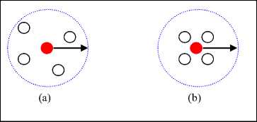
Fig.1. Local Density based on accumulating of distances to 4 ^th nearest neighbors

By examine Fig.1a and 1b both central red points have the same number of points in their fixed neighborhood span (the Eps is the same as used in DBSCAN) but local density of red point in Fig. 1b is greater than the local density of the red point in Fig. 1a. The totals of separation distances express this reality precisely. But in light of fixed Eps neighborhood span as in DBSCAN method there is no distinction, because each point has the same number of points in its Eps radius. And it is easy to note that, the value of Eps differs according to the local density depending on the totals of separation distances to the k- nearest neighbors, the points in core of cluster have high density (small total separation distances), on the other hand the points at the edge (border) of cluster have low density(large total separation distances), since the neighbors for this points exist in one side of it, but the points at the core of cluster have their neighbors inclosing them from all direction. So density depended on accumulating separation distances is more suitable than enumerating the points in fixed Eps distance.

• B.    Density Rank of Points

After calculating local density of each point in dataset using function (3), the algorithm calculates the density rank of each point. The density rank refers to the ability of point to attract its neighbors. The two red points in Fig. 2 attracts all their neighbors, the black point attracts zero neighbor. We can classify points as attractors and attracted. If the density of a point p is higher than the density of all its k -nearest neighbors then p is pure attractor as the case of red points in Fig. 2. Attractor point is the point that attracts points more than threshold; we will refer to it as minpts.

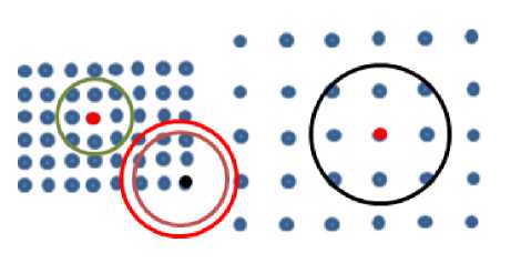
Fig.2. The two red points have max density rank, the black point has smallest density rank

The cluster here will be composed of attractors and attracted points. The black point is pure attracted, it attracts zero point of its k -nearest neighbors since it has the lowest density among it k -nearest neighbors, but it is attracted to attractor, therefore it is assigned to its cluster. We can call all attracted points that are not attractors “border points”. Noise point is the point that is not attractor and not attracted to any attractor.

The density rank of point p counts the attracted points to p. all the attracted points have lower density than that of p. Since the density of points is calculated as sum of distances to neighbors, so you find that the smaller the distance the higher the density of point is and vice versa, mostnear is another threshold. The density rank is calculated mathematically as in formula (4).

Density _ Rank ( p ) = q_j ∈ k_nn ( p_i )

Density ( p ) ≤ Density ( q )

In dense regions you find that the distances between points are small and vice versa in sparse regions the distances between points are large. You find a reverse proportional relationship between the density of point and the distances between itself and its neighbors. In density regions the density of point according to the density function shown in relation (3) is smaller than that in sparse regions. For any two different points, the algorithm gets the same number of neighbors. So as the accumulated distances between the point and its neighbor’s increases, the sparser the region the point lies in is. On the other hand, the smaller the accumulated distances is the denser the region is.

As the density of point increase its density rank increase and the vice versa. The density rank of any point will range from 0 to k , where k refers to number of k -nearest neighbors as in (5).

0 ≤Density_Rank(pi) ≤ k (5)

So the densest point p in any cluster has the largest value for Density Rank that will be equal to k . Keep in mind that the densest point has the smallest total of separation distances to its k -nearest neighbors. This is shown in Fig. 3. The red points have the smallest Density Rank in their clusters and the blue points have the largest Density Rank, where k is equal to 7.

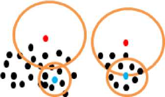
Fig.3. Blue points are the densest points in their clusters and have the largest value for Density Rank in their clusters

• C.    The Proposed Algorithm

The algorithm calculates the local density for each point p using function (3), and the Density Rank using function (4), then orders the points in dataset in descending order according to the local density of each point using the quick sort method. So the first point in the list will be the densest one in data space and the last one will have the lowest density. And then starts creating clusters beginning with densest points first, i.e. it moves from densest region to sparser one.

As in DBSCAN algorithm, the proposed algorithm uses the Density Rank in expanding clusters. If Density

Rank of point p is larger than threshold then this point is added to seed list to retrieve its neighbors. Otherwise it is assigned to the current cluster because it is within k 1 -nearest neighbors of current point that has density rank larger than the threshold minpts . The point with the smallest density comparing with its neighbors is considered as noise temporary; this point will have density rank equal to zero or less than or equal to minpts . The algorithm considers any point with density rank less than four as noise temporary. This condition look likes core point condition in DBSCAN algorithm. The following lines describe the proposed algorithm:-

CBLDP (data, k , k 1, mostnear , minpts )

Clus_id=0

FOR i =1 to size of data

Density(data[i], mostnear )=sum of distances between data[i] and its mostnear neighbors.

Desity rank of data[i]=number of points that are less dense than data[i] among its k -nearest neighbors.

NEXT i

Sort data point in ascending order based on Density (data points, mostnear )

For i =1 to size of sorted data

Maxdensity = the density of densest point among current_point and its k -nearest neighbors

Mindensity = the density of lowest dense point among current point and its k -nearest neighbors IF (current_point is unclassified and its density rank > minpts ) THEN Clus_id=clus_id +1

Expand_cluster(data, current_point, k , k1 , minpts , clus_id)

ENDIF

NEXT i

All unclassified points in data are noise

END CBLDP

Expand_cluster(data, current_point, k , k 1, minpts , clus_id) Seed=current_point

Neighbor = current_point.regionquery(current_point, k )

For x =1 to k

IF (current_point. Neighbor( x ) is unclassified) THEN

Assign it to the current cluster clus_id

IF (density of current_point.Neighbor(x) within Maxdensity and Mindensity and its density rank >  minpts THEN

Append current_point.Neighbor(x) to seed. END IF

END IF

NEXT x

Seed .delete(current_point)

While seed< > empty do point=seed.getfirst Neighbor= point.regionquery (point, k 1 ) Update Maxdensity and Mindensity according to max and min density of point and its minpts neighbors.

For x =1 to k 1

IF (point.Neighbor(x) is unclassified) THEN Assign it to the current cluster clus_id

IF (density of point. Neighbor(x) within Maxdensity and Mindensity and its density rank >  minpts THEN Append point.Neighbor(x) to seed.

END IF

END IF

NEXT x

End while

End Expand_cluster

The proposed algorithm uses four thresholds as shown in Fig. 4; k , k 1 , mostnear , and minpts .

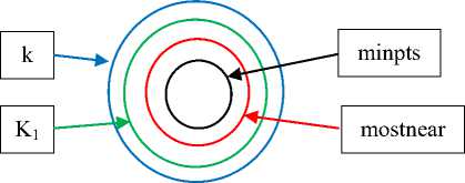
Fig.4. The relation between the four thresholds used in the proposed algorithm

Minpts is used in similar way as in DBSCAN. It is used in comparing with density rank of each point. If the density rank of a point p is larger than minpts , then the point p is a core point otherwise it is considered as noise temporary. Also it is used in updating maximum density and minimum density allowed in the cluster by small value to avoid splitting cluster. And this threshold is fixed to four by experiments.

Mostnear is used in finding local density of each point. Not all points in data space affect to local density of a point p but only few points affect to local density of a point, this parameter is called mostnear in the proposed algorithm and its value ranges from 4 to 8 by experiments. i.e 4 ≤ mostnear ≤ 8.

k is used to determine the size of neighbors of each point, 15 ≤ k ≤ 50 by experiment. This parameter is used in finding density rank of each point, also for the first point in each cluster to add all unclassified k-nearest neighbors to seed list, because the first point is usually the densest point in its cluster, and is pure attractor. It is used also in determining the initial values for maximum density and minimum density allowed in the cluster.

K 1 is used to determine the size of neighbors of each point (attractor) in the cluster except the first point in the cluster. So the algorithm avoids merging clusters with large varied density, in other word to discover cluster with varied density, 11≤ k 1 ≤ k by experiments.

• D.    Time Complexity

The time complexity of the proposed algorithm is similar to that of DBSCAN algorithm. To compute the local density of n point, the algorithm retrieves the k-nearest neighbors for each point, if the algorithm use the R* tree this operation requires (n log n). The algorithm also needs to sort the points according to their local density, if the algorithm use the quick sort method, this operation requires (n log n). These two operations are the most time consuming. So the average time complexity of the proposed algorithm is o(n log n).

• IV.    Experimental Results

This section presents some experiments of the proposed algorithm on some different synthetic datasets used in the area of clustering research. These datasets have clusters with different shapes, sizes, and densities. The algorithm discovers the actual clusters.

DS5

DS8

DS7

DS9

DS10

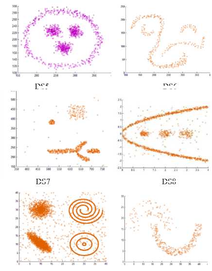
Fig.6. Datasets borrowed from [24]

DS6

DS1(8000)                   DS2(8000)

DS3(8000)                  DS4(10000)

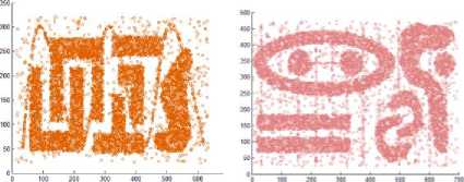
Fig.5. Some artificial datasets used to evaluate clustering algorithms by some researchers

The proposed algorithm is implemented in C++. We have utilized the artificial datasets that were utilized as a part of [16] to check the proposed algorithm. We tested the algorithm by applying it on four disparate datasets consists of points in two dimensional spaces whose geometric shape are presented as in Fig. 5.

The first dataset, DS1, includes six bunches of dissimilar shape, size, and orientation, and additionally arbitrary noise points and special chain such as streaks running crosswise over bunches.

The second dataset, DS2, contains nine groups of various orientation, size, and shape; two of them are within the space surrounded by other cluster. Moreover, DS2 also has arbitrary noise and special artifacts, such as a series of points forming vertical streaks. The third data set, DS3, has eight groups of varied size, shape, density, and orientation, in addition to arbitrary noise points. A specifically strenuous feature of this dataset is that bunches are very close to each other and they have varied densities. Finally, the fourth dataset, DS4, consists of six clusters of varied shape linked by density streak of points. The first three datasets are of the same size, each of them contains 8000 points. The fourth dataset consists of 10000 points.

Also, we have utilized the artificial datasets that were used in [24] to inspect the proposed method. We tested the algorithm by applying it on additional six varied datasets consisting of points in two dimensional space whose geometric shape are as depicted in Fig. 6.

These datasets contain clusters with complex structure. DS5 includes 3 spherical shaped clusters in a circular cluster, a total of 1016 points. DS6 is composed of 4 varied clusters, a total of 315 points. DS7 consists of two spherical clusters, two manifold clusters and a few outliers, a total of 582 points. DS8 consists of 3 spherical clusters, one elliptical cluster and some noise points. DS9 is composed of 7 clusters with multi shapes and some noises, a total of 8573 points. DS10 is composed of two varied shape and density clusters, a total of 373 points.

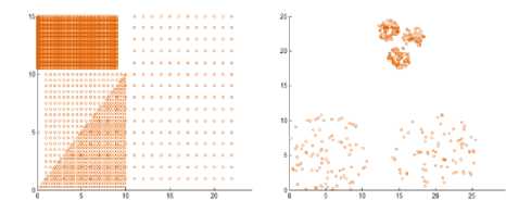
Also, we created two additional synthetic datasets including points in two dimensional space whose geometric shape are as depicted in Fig. 7 to evaluate the algorithm. DS11 contains 4 varied shapes, sizes, and dense clusters, a total of 3147. DS12 composed of 5 spherical clusters with large variance in size and density, contains 383 points.

DS11

DS12

Fig.7. Our synthetic datasets

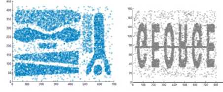
The clusters resulting from the proposed algorithms are shown in Fig. 8 that proves the efficiency of the proposed algorithm. The algorithm discovers the actual clusters in data. But there is a problem when two clusters with varied density are Siamese. This can be seen in dataset 11 where the denser triangle cluster takes some points from the low density triangle cluster that is attached to it.

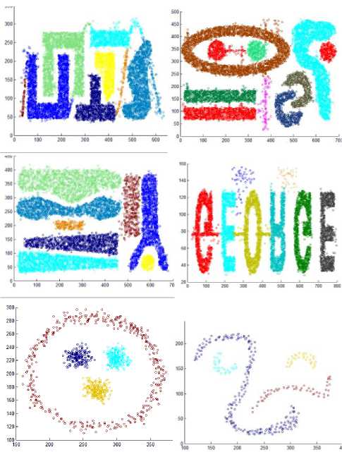
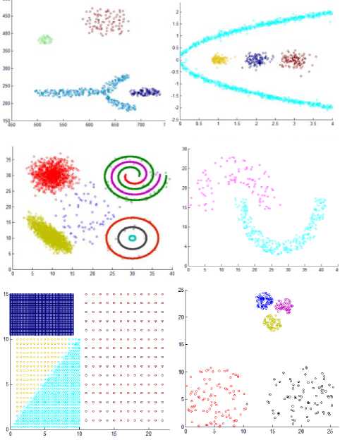
Fig.8. The results of the proposed algorithm.

The number of misclassified points is less than the k 1 -nearest neighbors used in the algorithm.

• V.  Conclusion

In this paper we have introduced a very simple idea to discover clusters with various shapes, sizes, and densities. The algorithm used only k -nearest neighbors to find local density of each point based on accumulating the distances to mostnear nieghbors that actually affects on. The algorithm specifies minimum and maximum density allowed in each cluster. The algorithm produces very good results as shown in Fig. 8. The algorithm requires three input parameters, these parameters need to be reduced as possible this what we will study in the near future work.

Acknowledgment

This project was supported by the Deanship of Scientific Research at Prince Sattam Bin Abdulaziz University under the research project no. 2017/01/7120.