A comparative investigation into edge detection techniques based on computational intelligence

Author: Naveen Singh Dagar, Pawan Kumar Dahiya
Journal: International Journal of Image, Graphics and Signal Processing @ijigsp
Article in issue: 7 vol.11, 2019.
Free access
Soft Computing becomes visible in the field of computer science. The soft computing (SC) comprises of several basic methods such as Fuzzy logic (FL), Evolutionary Computation (EC) and Machine Learning (ML). Soft computing has many real-world applications in domestic, commercial and industrial situations. Edge detection in image processing is the most important applications where soft computing becomes popular. Edge detection decreases the measure of information and filters out undesirable information and gives the desirable information in an image. In image processing edge detection is a fundamental step. For this, high level Computational Intelligence based edge detections methods are required for different images. Computational Intelligence deals with ambiguous and low cost solution. The mind of the human is the key factor of the soft computing. In this paper, we included Binary particle Swarm Optimization (BPSO), Distinct Particle Swarm Optimization (DPSO), Genetic Algorithm (GA) and Ant Colony optimization (ACO) techniques. The ground truth images are taken as reference edge images and all the edge images acquired by different computational intelligent techniques for edge detection systems are contrasted with reference edge image with ascertain the Precision, Recall and F-Score. The techniques are tested on 100 test images from the BSD500 datasets. Experimental results show that the BPSO provides promising results in comparison with the other techniques such as DPSO, GA and ACO.
Image processing, edge detection, ACO, GA, BPSO, DPSO, BSD500, F-Score
Short address: https://sciup.org/15016068
IDR: 15016068 | DOI: 10.5815/ijigsp.2019.07.05
Text of the scientific article A comparative investigation into edge detection techniques based on computational intelligence
In image handling and computer eyesight applications edge detection is a low dimension activity. The principle objective of edge detection is to find out the sharp discontinuities which are present in the image. These sharp discontinuities are present in the image due to abrupt changes in the intensity level in the image which describes the edges of the entities in the image. These boundaries are used to identify the objects for division and coordinating reason [1].These object boundaries are the initial phase in huge numbers of computer eyesight calculations like edge based face acknowledgment, edge based obstruction detection, edge based target acknowledgment, picture pressure and so forth. There are many edge detection methods are available [2].These detectors distinguishing vertical, flat, corner and step edges. The nature of edges recognized by these detectors is profoundly reliant on noise\commotion, lighting conditions, objects of same forces and the thickness of edges in the image [19, 20].
Computational intelligence has raised as an amazing asset for data handling, basic leadership, and knowledge the executives. The procedures of computational insight have been effectively created in territories, for example, neural systems, fluffy frameworks, and transformative calculations. It is unsurprising that sooner rather than later computational knowledge will assume a progressively imperative job in handling a few building issues. Picture handling is an imperative research zone [21]. Established picture preparing strategies frequently confront incredible troubles while managing pictures containing commotion and twists. In these cases, the utilization of computational knowledge approaches has been as of late reached out to address testing true picture handling issues [21].
The research motivation of this paper is to compare the different edge detection techniques which are based on computational intelligence. The four major categories of Computational Intelligence based techniques are BPSO, DPSO, ACO and GA. The mind of human is the imitation of these techniques which are based on biological content inspired by the nature. The above mentioned techniques are estimated for the same dataset classification. The 100 test images are taken from “BSD500” dataset for the implementation of the concept. For comparing the results, we are considering the accuracy performance parameters like “Precision, Recall and F-Score to get the best results in all scenarios. Rest of the paper is organized as follows: Section II gives the brief idea of related work; Section III gives the basics of Computational Intelligence techniques” considered for the edge detection; Section IV gives the experimental result and discussion; Section V gives the conclusion and future scope of the paper.
-
II. Related Work
Different sorts of operators are accessible for edge detection. Yet, these operators are classified into two classifications. In First order derivative [3] the information picture is convolved by an adjusted mask to produce a gradient picture in which edges are distinguished by thresholding. Most traditional operators like sobel, prewitt, robert [5] are the first order derivative operators. These operators are additionally said as gradient operators. These gradient operators identify edges by searching for greatest and least intensity values. These operators inspect the conveyance of intensity values in the area of a given pixel and decide whether the pixel is to be classified as an edge. These operators have more computational time and can't be utilized in real time application. In second order derivative [6], these depend on the extraction of zero crossing points which shows the nearness of maxima in the picture. In this, picture is first smoothed by an adaptive filters [4].Since the second order derivative is exceptionally sensible to noise, and the filtering function is critical. These operators are derived from the Laplacian of a Gaussian (LOG), and proposed by Marr and Hildreth [3], in this, the image is smoothed by a Gaussian filter. The field of soft computing was proposed by Dr. Lotfi Zadeh, with a goal to construct new generation Artificial Intelligence, known as Computational Intelligence [5, 6]. Soft Computing deals with imprecision, uncertainty, partial truth, and approximation to achieve practicability, robustness and low solution cost. Soft Computing in its latest incarnation as the fusion of the fields Fuzzy Logic, Neuro-computing, Evolutionary Computing, Genetic Computing, and Probabilistic Computing. The main goal of Soft Computing is to develop intelligent machines and to solve nonlinear and mathematically un-modeled system problems [5]. Soft computing techniques, which emphasize gains in understanding system behaviour in exchange for unnecessary precision, have proved to be important practical tools for many contemporary problems [2]. The applications of Soft Computing have proved two main advantages. First, it made solving nonlinear problems, in which mathematical models are not available, possible. Second, it introduced the human knowledge cognition, recognition, understanding, learning, and others into the fields of computing [6].
-
III. Different Computational Intelligence Techniques
In 1990 professor Nick Cercone gives the idea of Computational Intelligence in image processing [3]. Artificial intelligence is the main branch from where the computational intelligence is derived. It has the ability to learn, simplify the complex computational problem by its intelligence. It includes various intelligence techniques out of which four techniques are selected in this paper. These Computational Intelligence Techniques are briefed as below:
-
3.1 Particle Swarm Optimization (PSO)
PSO is a worldwide optimization technique which is inspired by the communal conduct of creatures and social model such as running of winged creatures and tutoring of fish [9]. PSO” was initially created to upgrade ceaseless nonlinear capacities; be that as it may, various alternative of particle swarm optimization have been given [10]. The population of people in particle swarm optimization is also called particles. Every particle in the population has its own mind so that they can keep information of the past states. PSO has effectively been utilized in numerous zones, for example, preparing neural systems [12], upgrading power frameworks [12], fluffy control frameworks [14], mechanical autonomy [22], radio and receiving wire plan [23], and PC diversions [14].
The fundamental PSO algorithm consists of n particles population which moves over an m -dimensional search space [9]. The Y j (t) gives the position of the j th molecule at time t which is defined as.
Y j (t) = ( y7 i (t),y7 2 (t),.......y7n(t)) (1)
The value of Y j (t) is upgraded with the help of particle influence and that of its neighbours. Y j is upgraded at each repetition of PSO by adding a velocity V j (t) [9], i.e.,
--* —* —* _ Y j(t+1) = Y (t) + V j (t+1) (2)
There are three main components by which the velocity can changed are current motion, particle memory and swarm influence, i.e. [9],
K j, i (t+1) = mK j i (t) + C 1 R and 1 ( Ypbest j^ -
-
Y j, i (t)) + C 2 R and 2 ( Y leader ц - Y j, i (t)) (3)
-
3.2 Binary Particle Swarm Optimization (BPSO)”
Where, Randi, and Rand2 are random variables whose value lies between 0 and 1. Here, m (idleness weight) which controls the effect of the past speed; C1 is known as self confidence and C2 is known as swarm confidence learning factors that speak to the fascination of a molecule toward either its own particular achievement or that of its neighbours; Ypbestj j means the best position of jth molecule up until this point; and Yleader is the situation of a molecule (the pioneer) used to direct different particles toward better areas of the pursuit space. The pioneer of every molecule is indicated by an associated neighbourhood topology [9, 11].
Despite the fact that “PSO” is normally connected to unconstrained optimization issues, different techniques for taking care of requirements have been given in “PSO”. These can be classified into four principle gatherings, protection, penalization, and preprocessing techniques. In the primary gathering, every single potential arrangement, spoken to by particles, are initialized to such an extent that they fall inside the workable inspection area, and specific administrators are connected so as to keep new arrangements from abusing existing requirements [10]. The second classes of algorithms are created to punish the wellness of the particles which are not set in an attainable territory [12]. Apportioning techniques isolate all particles into two sets: achievable set and impractical set. These strategies fix impractical arrangements or organize arrangements dependent on their possibilities [9]. Pre-processing strategies change the optimization issue into another with the end goal that either the imperatives can be taken care of in a less demanding way, or they can be disposed of [11].
The concept of BPSO is also given by Kennedy and Eberhart which allows BPSO to operate in binary space [13]. In BPSO, a new approach is suggested to update the position of particles which takes either 0 or 1 in d £h dimension as:
t+i = (° ifrandQ > Siglve^1)ld (1 if rand() < Sig(vel-+1)
Where, Sig(. ) is the sigmoidal function which is used to change the velocity component in between [0, 1]. The sigmoidal function can be expressed as:
Sia(vel t+1 ) =--- ~7+- (5)
1+e ve ‘id
Algorithm 1: Code for BPSO with a mutation [14]
Start t = 0; {t: show the index of generation} load the particles Y j, i(t);
evaluate Y j , i(t);
while(termination condition ≠ true)
do
-
V j, i (t) = upgrade V j, i (t); {by Eq. (1)}
-
V j, i (t) = alteration V j, i (t); {by Eq. (2)}
Y j, i (t) = upgrade Y j, i (t); {by Eqs. (4) and (5)} evaluate Y j ,i (t);
-
t = t + 1;
-
3.3 Distinct Particle Swarm Optimization (DPSO)”
end while
Stop
The cipher of “BPSO” is given in Algorithm 1. It ought to be noticed that the BPSO is helpless to sigmoid capacity immersion, which happens when speed the speed are too high or too low [19]. In such cases, the likelihood of an adjustment in bit esteem approaches zero, in this manner limits investigation and the likelihood of an adjustment in bit esteem approaches one expands misuse. For a speed of 0, the sigmoid capacity restores a likelihood of 0.5, suggesting that there is a half shot for the bit to flip. Be that as it may, speed bracing will defer the event of the sigmoid capacity immersion. Consequently, ideal determination of speed is critical for quicker intermingling [19, 14].
The new cipher strategy proves that the explore area is distinct\individual. Thus, when positions of the particle are upgrading, they require to be cut short to the integers. The proposed cut short method is given by:
b j
((bj + 1) mod 8 bj-[bjJ>^l { bj mod 8 otherwise J
[ ([afJ + 1) aj - [ajJ > ^1 mj ( [a,-J otherwise J where the value of N is a uniform arbitrary number chosen in between 0 to 1. Keeping in mind this rule does not utilize to upgrade the velocities of the particle as we want them to be accurately upgraded [14].
-
3.4 Brief Idea of Genetic Algorithm
During 1970s the genetic algorithm was first introduced by Holland [15, 16, 17], is a hypothetical hunt and optimization strategy which depends on the standards of normal natural development. Population is the method of genetic algorithm [15]. In the search space each particle is a solution in the population which is ciphered as chromosome and to compute the fitness of every particle the algorithm will repeat the following and select the particle with good result, crossover and mutation are done to reproduce the next generation [16]. The repetition will stop when the fitness average value of the total generation becomes relatively stable [15]. To detect an edge with the help of genetic algorithm is little bit different from the conventional one [17]. Each particle is an edge structure. Fig. I gives the idea of crossover operation. A random point is first selected and divides the 2-D array into four parts. The mutation operation selects the random genes and changed the bit [15].
-
3.4.1 “Genetic Algorithm Approach”
-
A. “Initialization”
At the beginning number of individual solutions are aimlessly produced to create an initial population.. Thousands of feasible solutions contains by the population [15]. Usually, the population is created aimlessly which covers the complete range of feasible solutions.
-
B. “Selection”
A relative amount of existing population is selected during each consecutive generation, and preserved for the new generation [15]. The scaled values of the fitness function selected the parents for the next generation. One step for each parent (equal step size) is moved along the straight line by this algorithm. The algorithm assigns a parent at each step. In the first step a uniform random number is assigned which is less than the step size [16].
-
C. Crossover
To produce a child solution a combination of parents is chosen. Many characteristics of its parents are shared by the new generation [15]. Two children from two parents are generated by the crossover operator which is chosen by the genetic algorithm solver. The selects vector entries from the first parent are less than or equal to n . The selects vector entries from the second parent is greater than n . The child vector is built by connecting these entries [17].
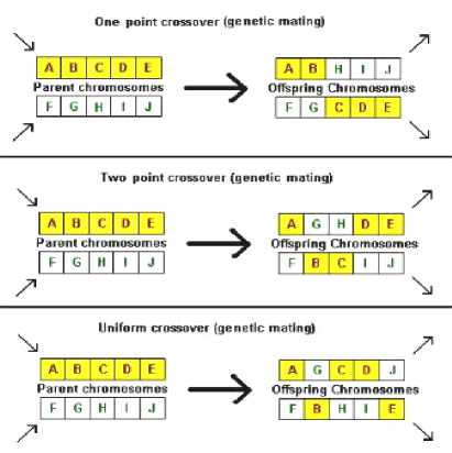
Fig.I. Crossover Operation
Let us take the example of two parents D1 and D2.
D1 = [a b c d e f g h] D2 = [9 8 7 6 5 4 3 2]
and point of crossover is 3, the following baby is produce by the function:
baby = [a b c 6 5 4 3 2]
The some part of the next generation is produced by crossover. The rest individuals in the next generation are produced by the mutation process [15].
-
D. “Mutation”
-
3.5 Ant Colony Optimization (ACO)
To produce a child solution a parent solution is selected. With random changes the same amount of information is shared by the new generation than its parents [15]. Although the main genetic operators are
“mutation and crossover other operators like migration and regrouping is also used in genetic algorithm. The active contour method is applied by the mutation function for the selected parents [16].
The source of inspiration for ant colony optimization (ACO)” is nature [6], for example ants behaviour\act that on moving from their house to the destination in search of food they deposit odor\scent which is also called pheromone on the ground to make some favourite paths so that the other ants of the colony can followed the same favourite path in search of the food. It is helpful for solving complex computational problems. The goal of the ant is to find the best preferred path for their destination in search of food [8]. The same phenomenon is accommodate by the ant colony optimization algorithm, artificial ants are formed which represent it as a software agent to find the best\optimal solutions to the given problem of optimization. The first ACO algorithm is given by Dorigo et al. [6]. ACO has been broadly connected in different issues [7].
ACO” intends to find best/optimal solution to the problem by guided search space over the arrangement space, by building the pheromone data. To be progressively explicit, assume absolutely Z ants are connected to locate the ideal arrangement in a space Y that comprises of B1 × B2 hubs, the technique of ACO can be condensed as pursues [6, 7]. “
-
• The pheromone matrix τ (0) and the positions of all Z ants are initialized.
-
• The construction-step index n = 1 : N, – For the ant index z = 1 : Z,
* The z-th ant are moved for L steps, in accordance with the probabilistic transition matrix T (n) successively (with a size of B1B2 ×B1B2 ).
– Now upgrade the pheromone matrix τ (n).
-
• The final pheromone matrix τ (n) helps to make the decision on the solution.”
In the above process there are two basic issues; that is, how to construct the probabilistic transition matrix T (n) and the matrix of pheromone τ (n) up-gradation, each of which is described as follow, respectively [6, 8].
In the first step of construction of ACO, with the help of probabilistic rule the zth ant moves from the i node to the j node, which is calculated by the following equation (8).
(n) _
1 i,j =
■ ъ^уУ^
if j e П ,
where t^” 1)is the information of pheromone value of the arc joining the node i to the node j; Ωi is the adjacent nodes for the ant az which is present on the node i; α and β are the two constants which gives the pheromone information and heuristic information respectively; the heuristic information from node i to node j is given by ηi,j, whose value is fixed for every construction step [6].”
In the second step of ACO, the pheromone matrix is upgraded two times in the whole ACO process [7]. The first upgrade is completed after the each ant movement; the pheromone matrix is upgraded by the equation 9 as:
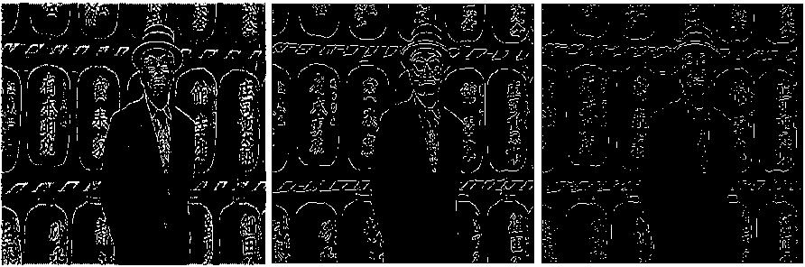
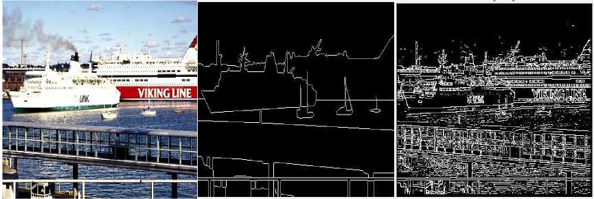
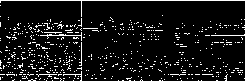
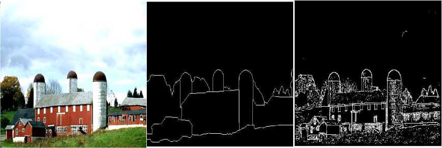
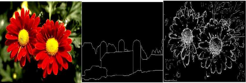
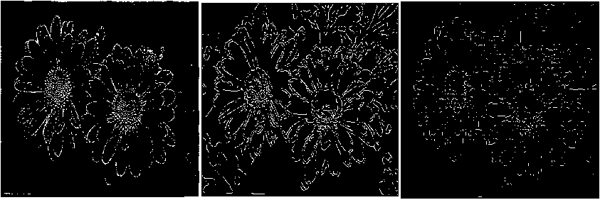
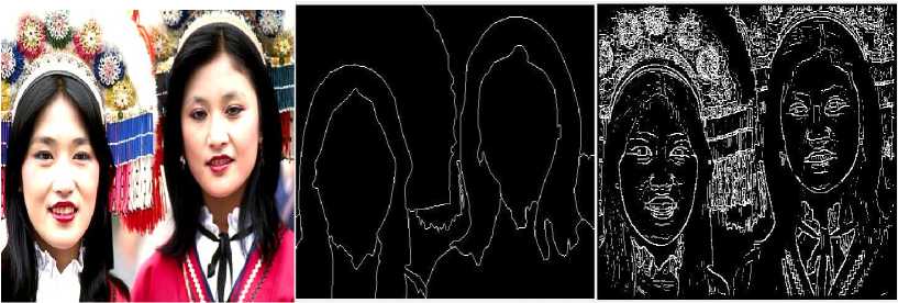
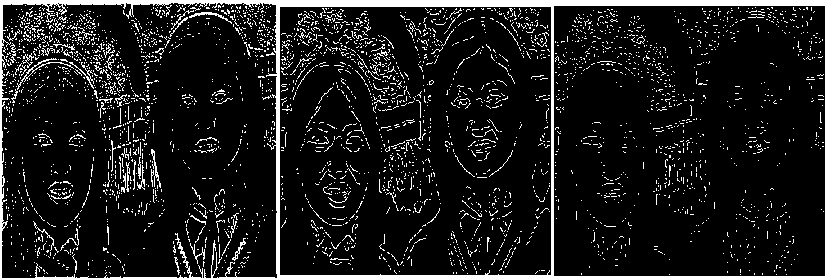
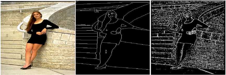
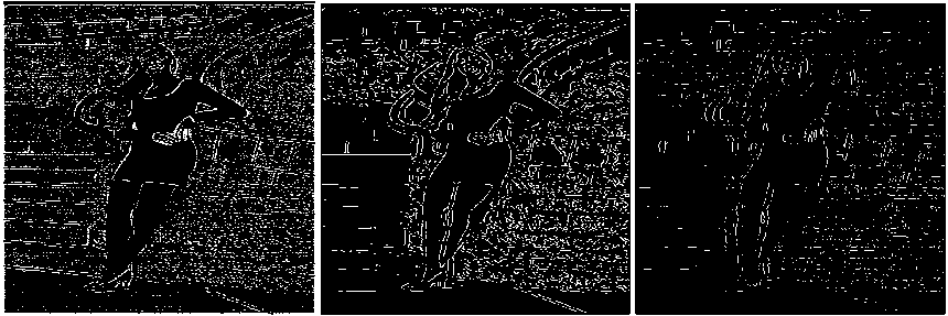
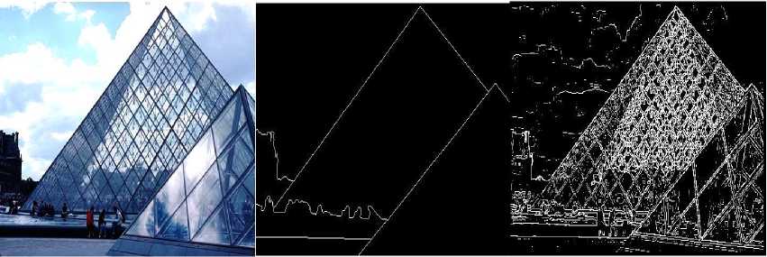
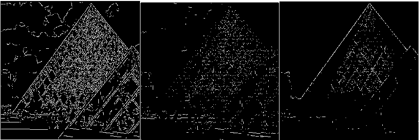
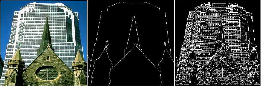
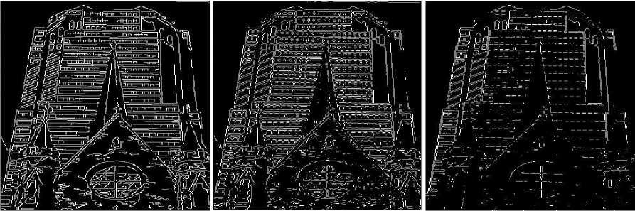
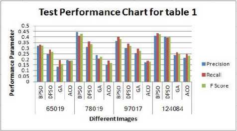
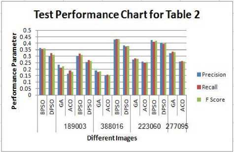
(n-1) _ 4j -х\1-р)лм + р-йи}> if (i,^belongs to the best tour = {т(П 1)}, otherwise (9) where ρ is the rate of evaporation. The best tour is found from the start of the algorithm [8]. In the each construction step the second upgrade is done after the movement of all Z ants and matrix of pheromone is upgraded by the equation 10:” τ(n) = (1 - ψ) · τ(n-1) + ψ · τ(o), (10) where ψ is the pheromone coefficient of decay. Note that the two upgrade operation are performed in ant colony optimization which are given by equation 9 and 10 respectively but the ant system performed only one upgrade which is given by equation 10 only.” IV. Experimental Result And Discussion The four major categories of Computational Intelligence based techniques are compared which are BPSO, DPSO, ACO and GA. All above techniques are compared for the same dataset classification [9]. The 100 test images are used from “BSD500” dataset for the implementation of the concept. For comparison, we are taking the accuracy performance parameters like “Precision, Recall and F-Score” to get the different feature results in all perspective. We have taken eight images from the BSDS500 datasets. Images are numbered as 65019, 78019, 97017, 124084, 189003, 388016, 223060 and 277095 respectively and the images are partitioned to obtain the ground truth images for reference edge images. The Ground truth images are taken from the BSD500 dataset. To get the idea how the ground truth images are computed we may refer the paper [9] in the references. In the figure 1 the original image (65019) as well as all the images detected by the different techniques is shown below: (a) (b) (c) (d) (e) (f) Fig.1 (a) Image 65019 (b) Ground Truth Image (c) BPSO (Binary Particle Swarm Optimization) (d) DPSO (Distinct Particle Swarm Optimization) (e) GA (Genetic Algorithm) (f) ACO (Ant Colony Optimization)” In the figure 2 the original image (78080) as well as all the images detected by the different techniques is shown below: (a) (b) (c) (d) (e) (f) Fig.2 (a) 78019 Image (b) Ground Truth Image (c) BPSO (d) DPSO (e) (e) GA (Genetic Algorithm) (f) ACO In the figure 3 the original image (97017) as well as all the images detected by the different techniques is shown below: (a) (b) (c) (d) (e) (f) Fig.3 (a) Image 97017 (b) Ground Truth Image (c) BPSO (Binary Particle Swarm Optimization) (d) DPSO (Distinct Particle Swarm Optimization) (e) GA (Genetic Algorithm) (f) ACO (Ant Colony Optimization)” In the figure 4 the original image (124084) as well as all the images detected by the different techniques is shown below: (a) (b) ( c) (d) (e) (f) Fig.4 (a) 124084 Image (b) Ground Truth Image (c) BPSO (d) DPSO (e) GA (Genetic Algorithm) (f) ACO In the figure 5 the original image (189003) as well as all the images detected by the different techniques is shown below: (a) (b) (c) (d) (e) (f) Fig.5 (a) Image 189003 (b) Ground Truth Image (c) BPSO (Binary Particle Swarm Optimization) (d) DPSO (Distinct Particle Swarm Optimization) (e) GA (Genetic Algorithm) (f) ACO (Ant Colony Optimization)” In the figure 6 the original image (388016) as well as all the images detected by the different techniques is shown below: (a) (b) ( c) (d) (e) (f) Fig.6 (a) 388016 Image (b) Ground Truth Image (c) BPSO (d) DPSO (e) GA (Genetic Algorithm) (f) ACO In the figure 7 the original image (223060) as well as all the images detected by the different techniques is shown below: (a) (b) ( c) (d) (e) (f) Fig.7 (a) 223060 Image (b) Ground Truth Image (c) BPSO (d) DPSO (e) GA (Genetic Algorithm) (f) ACO In the figure 8 the original image (277095) as well as all the images detected by the different techniques is shown below: (a) (b) ( c) (d) (e) (f) Fig.8 (a) 277095 Image (b) Ground Truth Image (c) BPSO (d) DPSO (e) GA (Genetic Algorithm) (f) ACO”” The test performance table for different techniques is given below. In which the value of performance parameters such as precision, recall and F score is calculated. Table 1. Test Performance (F, Recall and Precision) for BPSO, DPSO, ACO and GA on first four Images” Image Techniques Precision Recall F Score 65019 BPSO 0.3178 0.3322 0.3248 DPSO 0.2462 0.2857 0.2645 GA 0.1345 0.1958 0.1595 ACO 0.1957 0.1851 0.1903 78019 BPSO 0.4421 0.4132 0.4272 DPSO 0.3126 0.3578 0.3337 GA 0.2364 0.2074 0.2209 ACO 0.1478 0.1879 0.1655 97017 BPSO 0.3647 0.3991 0.3811 DPSO 0.2987 0.3378 0.3171 GA 0.2536 0.2953 0.2729 ACO 0.1725 0.1851 0.1786 124084 BPSO 0.4128 0.4337 0.4229 DPSO 0.4013 0.3953 0.3982 GA 0.2374 0.2627 0.2494 ACO 0.2136 0.2481 0.2296 The test performance chart for table 1 shows in fig.9. From the graph we conclude that the Binary particle Swarm Optimization (BPSO) techniques gives the best value of performance parameters as compared to the other techniques. Fig.9. Test Performance Chart for Table 1. The test performance of next four images are shown in the table 2. In which the value of performance parameters such as precision, recall and F score is calculated. The test performance chart for table 2 shows in fig.10. From the chart we conclude that the Binary particle Swarm Optimization (BPSO) techniques gives the best value of performance parameters as compared to the other techniques. Table 2. Test Performance (F, Recall and Precision) for BPSO, DPSO, ACO and GA on next four Images Image Techniques Precision Recall F Score 189003 BPSO 0.3647 0.3534 0.3589 DPSO 0.3014 0.3219 0.3113 GA 0.2346 0.2114 0.2224 ACO 0.1654 0.1880 0.1759 388016 BPSO 0.3014 0.3177 0.3094 DPSO 0.2547 0.2685 0.2614 GA 0.1897 0.1765 0.1828 ACO 0.1486 0.1578 0.1531 223060 BPSO 0.4278 0.4325 0.4301 DPSO 0.3846 0.3751 0.3797 GA 0.2762 0.2814 0.2787 ACO 0.2603 0.2513 0.2557 277095 BPSO 0.4235 0.4136 0.4185 DPSO 0.4025 0.3975 0.3991 GA 0.3247 0.3364 0.3304 ACO 0.2568 0.2632 0.2598 Fig.10. Test Performance Chart for Table 2 The 100 test images are used from “BSD500” dataset for the implementation of the concept and it is impossible to show the entire images in the paper that’s why we are calculating the mean and standard deviation of all techniques for all performance parameters. Table 2. “Average test performance of all edge detectors on 100 BSD test images Techniques “Precision (Mean ± Std)” “Recall (Mean ± Std)” “F-score (Mean ± Std)” BPSO 0.3457 ± 0.0531 0.3614 ± 0.0794 0.3568 ± 0.0701 DPSO 0.2743 ± 0.0711 0.3347 ± 0.0568 0.2987 ± 0.0519 ACO 0.1987 ± 0.1025 0.2258 ± 0.0974 0.2214 ± 0.0961 GA 0.1568 ± 0.0625 0.1857 ± 0.0610 0.1657 ± 0.0673 Mean and standard deviation of all approaches when tested on 100 BSD test images are shown in Table 2. It is also clearly visible from Table 2 that BPSO also outperforms all other edge detection techniques when tested on 100 test images. V. Conclusion/Future Scope The paper gives the comparative investigation of edge detection techniques which are based on computational intelligence. We are comparing four different techniques named as Binary Particle Swarm Intelligence (BPSO), Distinct Binary Particle Swarm Intelligence (DPSO), Ant Colony Optimization (ACO) and Genetic Algorithm (GA) which are based on human mind Modelization, biological content inspired by nature and other intelligent classifiers. The ground truth images are taken as reference edge images and all the edge images acquired by different computational intelligent techniques for edge detection systems are contrasted with reference edge image with ascertain the Precision, Recall and F-Score. The techniques are tested on 100 test images from the “BSD500” datasets. Experimental results show that the BPSO provides better results in comparison with the other techniques such as DPSO, GA and ACO. Experimental results indicate that the Computational Intelligence based techniques actively increases the edges of the image as compared to the conventional techniques such as “Robert, prewitt, Sobel and Canny” but the processing time taken by computational techniques are much more than the conventional techniques thus reducing the processing time is future study.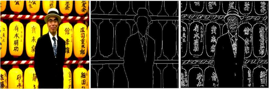

References A comparative investigation into edge detection techniques based on computational intelligence
- L. S. Davis, “A Survey of Edge detection Techniques”, Computer Graphics and Image Processing (1975) 4, (248-270).
- D. Marr & E. Hildreth, “Theory of edge detection”, Proc. R. Soc. London B207, 187-217 (1980).
- T. Peli & D. Malah, “A study of edge detection algorithms”, Computer Graphics and Image Processing 20, 1-21 (1982).
- V. Torte & T. A. Poggio, “On edge detection”, IEEE Trans. Pattern Anal. Mach. Intell. PAMI-8, 147-163 (1986).
- N. S. Dagar, P. K. Dahiya, “Soft Computing Techniques for Edge Detection Problem: A state-of-the-art Review”, International Journal of Computer Applications (0975 – 8887) Volume 136 – No.12, February 2016.
- N. S. Dagar, P. K. Dahiya, “A Comparative Analysis of Edge Detection Algorithm and Performance Metric Using Precision, Recall and F- Score”, International Journal of Modern Electronics and Communication Engineering (IJMECE) ISSN: 2321-2152 Volume No.-6, Issue No.-6, November, 2018.
- H. Nezamabadi, S. Saryazdi & E. Rashedi, “Edge detection using ant algorithms”, Soft Computing (2006) 10: 623–628 DOI 10.1007/s00500-005-0511-y Published online: 1 August 2005 © Springer-Verlag 2005.
- J. Tian, W. Yu & S. Xie. "An ant colony optimization algorithm for image edge detection", IEEE Congress on Evolutionary Computation (IEEE World Congress on Computational Intelligence), 2008.
- P. Arbelaez, M. Maire, C. Fowlkes and J. Malik, “Contour Detection and Hierarchical Image Segmentation”, IEEE Transactions on Pattern Analysis and Machine Intelligence, volume 33, issue-5, May 2011.
- J. Tian & W. Yu., "Ant-Inspired Visual Saliency Detection in Image", IGI Global, 2011.
- M. Setayes, M. Zhang & M. Johnston, “Edge Detection Using Constrained Discrete Particle Swarm Optimisation in Noisy Images”, IEEE 978-1-4244-7835-4/11/$26.00 ©2011 IEEE.
- J. Kennedy & R. Eberhart, “Particle Swarm Optimization”, IEEE 0-7803-2768-3/95/$4.00 0 1995 IEEE.
- M. Braik, A. Sheta & A. Ayesh, “Image Enhancement Using Particle Swarm Optimization”, Proceedings of the World Congress on Engineering 2007 Vol 1, WCE 2007, July 2 - 4, 2007, London, U.K.
- A. Gorai, & A. Ghosh, “Gray-level Image Enhancement by Particle Swarm Optimization”, IEEE 978-1-4244-5612-3/09/$26.00c 2009 IEEE.
- S. Lee, S. Soak, S. Oh, W. Pedrycz & M. Jeon, “Modified binary particle swarm optimization”, National Natural Science Foundation of China and Chinese Academy of Sciences. Published by Elsevier Limited and Science in China Press 2008.
- I. Lovrek, R. J. Howlett & L. C. Jain, "Knowledge-Based Intelligent Information and Engineering Systems", Springer Nature America, Inc, 2007.
- N. Senthilkumaran, “Genetic Algorithm Approach to Edge Detection for Dental X-ray Image Segmentation”, International Journal of Advanced Research in Computer Science and Electronics Engineering (IJARCSEE), Volume 1, Issue 7, September 2012.
- S. M. Bhandarkar, Y. Zhang & W. D. Potter, “An Edge Detection Technique Using Genetic Algorithm-Based Optimization”, Pattern Recognition, Vol. 27, No. 9, pp. 1159 1180, 1994 Elsevier Science Ltd Copyright © 1994 Pattern Recognition Society.
- W. Fu, M. Johnston & M. Zhang, “Low-Level Feature Extraction for Edge Detection Using Genetic Programming”, IEEE TRANSACTIONS ON CYBERNETICS, Vol. 44, No. 8, august 2014.
- S. L. Gupta, A. S. Baghel & A. Iqbal, "Threshold Controlled Binary Particle Swarm Optimization for High Dimensional Feature Selection", International Journal of Intelligent Systems and Applications, 2018
- E. Cuevas, D. Zaldívar, G. Pajares, M. P. Cisneros & R. Rojas, "Computational Intelligence in Image Processing", Mathematical Problems in Engineering, 2013.
