A Comparison of Simpson’s Rule Generalization through Lagrange and Hermite Interpolating Polynomials

Numerical integration methods for unequally spaced data have been studied in various fields. Researchers have proposed formulas using techniques like Newton’s Divided Difference formula to derive quadrature formulas, such as Trapezoidal and Simpson’s rules, for unevenly spaced data [1 ， 2]. Additionally, in the context of time-series analysis, models like the complex irregular autoregressive model have been introduced to efficiently fit irregularly spaced time series data, allowing for accurate parameter estimation and forecasting of unobserved measurements [3]. Moreover, in spatial data analysis, a method based on Fourier transform has been described to approximate multiple integrals of covariance functions over irregular data regions with high accuracy and reduced computational cost [4]. These diverse approaches offer valuable tools for handling numerical integration with unequally spaced data. New interpolation, numerical differentiation, and numerical integration formulas with arbitrary order of accuracy are derived for evenly and unevenly spaced data [5].

Simpson's Rule is a widely used method for numerical integration, known for its accuracy and efficiency in approximating definite integrals. It is particularly well-suited for situations where the integrand is known only at a set of discrete points [6]. However, the accuracy of Simpson's Rule relies on the assumption of equally spaced data points, a condition that is often violated when dealing with real-world data [7,8]. This limitation arises due to various factors such as limitations in measurement techniques, the nature of the phenomena being studied, or constraints imposed by experimental setups.

Researchers have explored several approaches to adapt Simpson's Rule for unequally spaced data. One common strategy involves interpolating the given data to generate a new set of equally spaced points before applying Simpson's Rule [9]. Another approach involves modifying Simpson's Rule itself to directly account for the unequal spacing of data points [10]. This typically entails adjusting the weights assigned to each data point in the formula to reflect the varying distances between them. While research has explored modified Simpson's Rules and compared their accuracy and efficiency against other techniques like the Trapezoidal Rule and Gaussian quadrature [11,12], these modifications can often be complex and may not always yield significant accuracy improvements, particularly for functions with substantial curvature.

Despite these efforts, a robust and accurate method for applying Simpson's Rule to unequally spaced data, particularly for functions exhibiting significant curvature, remains a significant challenge in numerical analysis. To address this gap, this paper presents a new generalization of Simpson’s Rule using both Lagrange and Hermite interpolating polynomials. These polynomial-based approaches provide a more flexible and potentially accurate way to handle unevenly spaced data while preserving the core principles of Simpson's Rule.

To provide a deeper understanding of my approach, I present a new geometric interpretation of Simpson's Rule, demonstrating its relationship to the area calculation of a trapezoid and a triangle. This interpretation reveals how the accuracy of the method is primarily linked to the chosen interpolation method for determining a crucial midpoint within each subinterval.

This paper conducts a rigorous comparative analysis of the accuracy and stability of Simpson's Rule generalized through both Lagrange and Hermite interpolating polynomials. By applying these methods to a diverse set of functions, including those exhibiting significant curvature, I demonstrate the strengths and limitations of each approach, particularly as the number of data points increases. Our analysis pays particular attention to error behavior, computational cost, and sensitivity to data distribution.

The findings of this research have important practical implications for any field that relies on accurate numerical integration of unequally spaced data. I discuss the potential benefits of my generalized Simpson's Rule methods in areas such as experimental data analysis, numerical simulation, and modeling of physical phenomena. Furthermore, I highlight the need for careful consideration of data characteristics and accuracy requirements when selecting the most appropriate interpolation method for a given application.

This research underscores the need for accurate and efficient numerical integration methods tailored for unequally spaced data, a challenge becoming increasingly prevalent in our data-driven world. The proposed Lagrange and Hermite-based generalizations of Simpson's Rule provide a valuable contribution to this effort, offering a balance of accuracy, efficiency, and applicability to a wide range of functions and scientific domains. Further exploration of adaptive algorithms holds promise for extending the impact of these methods to the increasingly large and complex datasets encountered in modern research and applications.

2.    Preliminaries 2.1.    Simpson’s Rule

Let a = x₀< x1 ... < x_2m = b , where x_k = x₀ + kh and let f_k = f (x_k) 0 < к < 2m . Then, the generalized Simpson’s rule is [13]

4^й f(x)dx = 1 (f₀ + 2 E E-i f_2k + 4 E m-i f_2k - _r + f_2m)                       (1)

• 2.2.    Lagrange Interpolating Polynomial

The Lagrange interpolation polynomial is a degree n polynomial that goes through (n + 1) points y₀ = f(x₀), У 1 = f(x 1 ), ......, y_n = f(x_n) It can be expressed as follows [14]

n

P^{(x) =} ^^p j (x)

J=o

Where n      n x -xk xJ - xk

^p j ^(x) = ^y j ⁿ J=0   k=0,k*J

• 2.3.    Hermite Interpolating Polynomial

Theorem 1. If f E C 1 [a,b] and x₀, .. ,x_n E [a,b] are distinct, the unique polynomial of least degree agreeing with f and f' at x₀,...., x_n is the Hermite Polynomial of degree at most 2n + 1 given by [15]

p(x) = E n=0 U_l(x)f(x_l) + E n=0 v_i(x)f ' (x_i)                                 (2)

where U (x) and V( (x) are polynomials in x of degree (2n + 1), which can be obtained as follows

/ л _ f0 when i * j; V^x) = 0 for all i

^{1 j} Ц when i = j

U'i(xj) = 0 for all i; V(xj) = {0 when \ * j’ iy >J              1 jj ц when i = j

So, now we can say

U i (x) = X i (x)[£ i (x)]²; V i (x) = B i (x)[L i (x)] ²

where

_Lr_x)_ (x - XoXx - x f )(x-x_n)

¹       (x i - xo'Kx i - xj(x i -x n )

Since the polynomial [L₁(x)]² has a degree of 2n and U₁(x) and V₁(x) have a degree of (2n + 1), it follows that A_i(x) and B₁(x) are both linear equations. Therefore, we can write

U i (x) = (a i + b i x)^[L i (x)^]2}

V_i(x) = (c_i + d_ix)[L_i(x)] ² }

From (4) and (4), we obtain

a₁ + b₁x = 1,c₁ + d₁x = 0 b₁ + 2L'₁(x₁) = 0,d₁ = 1

'}

By solving equations in (5) , we get

^b i = ^c i =

—2L ' ₁(x₁),a₁ = 1 + 2x_iL'₁(x_l)

—xi , d i = 1

}

Substitute values in (6) in (4)

U i (x) = (1 - 2(x-x i )L' i ⁽x i ⁾)^[L i ⁽x^{)] 2}

}

V i (x) = (x-x_i)^[L i (x)] ²

Finally, by substituting U₁(x') and V₁(x) into (2), we get

n

n

P⁽x) = ^(1 — 2(x—x i )L' i ⁽x i ⁾)^[L i ⁽x^{)] 2} f⁽x i ⁾ + ^⁽x-x i ^)[L i ⁽x^{)] 2} f ' (x i )

1=0

i=0

3.    Main Results

Proposition 1 . For any three points (x₀,y₀), (x_i,y_i), and (x₂,y₂) the area (A) of the triangle formed by these points is given by the formula

A = ^ ^[x o ⁽y 2 — У 1 ) + x 1 ⁽y o - У 2 ) + x 2 ⁽y i - У о ^)]

Proof. Consider a triangle AABC in the Cartesian plane, where A(x₀,y₀), B(x_i,y_i), and C(x₂,y₂) are its vertices. Let N, M, and L be the x-axis points, and 0 is the origin.

Then NM = 0M - ON = x_i - x₀ , NL = 0L - ON = x₂ - x₀, and ML = 0L - 0M = x₂ - x_i. Now, we express the area A as the sum of the areas of these trapeziums

A = - [(AM + BN) x NM + (AM + CL) x ML - (BN + CL) x NL]

= 2 ^[(y i + y o )(x i - x o ) + ⁽y i + y2)(x 2 - x i ) - ⁽y o + y2)(x 2 - x o )^]

= 2 ^[x o ⁽y 2 - y i ) + x i ⁽y o - y 2 ) + x 2 ⁽y i - y o ^)]

Theorem 2. Let P (x) be a polynomial with a degree of three or lower that is defined on the interval [a, b]. Let A, B, and C be different points on the curve у = P(x) Denote the midpoint of the interval by C. If A_t represents the total area enclosed by the curve у = P(x) and the line segments AC and BC, then it holds that

A_t = i .Ar ea(AAB C)

And the area under the curve

f a f⁽x) dx = ^^[f⁽a') + f⁽b^)] + ⁴ A

Where A is AABC area

Proof. Consider a polynomial P(x) of degree three or lower defined on the interval [a, b]. Let A = (x_i,f(x_i)),

B = (x₂,f(x₂)), and C =

interval [a, b] is

X X i +X - f X X 1 +X₂ ^

be three different points on the curve у = P(x) The total area over the

^X 2                 ^X 2

A_t = I f(x)dx = I [a₀x ² + a_ix +

X 1                X 1

a₀x ³ a_ix²

a2\dx = l~^~ + ~^~ + « 2 x1

X 2

= (^)« o + (^)

a i + a₂(x₂

—

x i )

X 1

We get the area of AABC from proposition 1

1 xi + x2

^A=-2^{[     2}

. x i + x 2

. x i + x 2

(f(x i ) — f(x 2 )) + x i (f(x 2 ) — f(

■ ))+x 2 f

■) — f(x i ))]

rf x i + x 2

[

—

x₂] ⁽a o x i ²

+ aixi

^{+ a}2^ ^{+ [x} i

—

x i + x 2

■ ] ⁽ O q x 2 ²

+ a i x 2 + a 2 )

ГГ x i

+ ^[x 2

—

x i ^]

(Ч^+Ч^^^

[

—

—] (a₀x_i² + a_ix_i + a 2 ) +

+ ^[x 2

—

x i ^]

x x i

—

—] ⁽a o x2² +

a i x 2 + O b )

^x i +^x 2 ^{2        x} i + ^x 2

(^a ° [-^)     (  2  ^"^ )

.

a o [x i³

_ 1 T2xi

=41

—

i

i

—

—

^a o

—

x₂)(a₀x_i ² + a_ix_i + a 2 ) + (x_i

+2^[x 2

—

—

x2')(a0x22 +

x^^)^

x₂)(a₀x_i ² + a_ix_i + a 2 ) + (x_i

+ ^[x 2

—

' x i + x 2

² + a i x 2 + a 2 )l '^{) + a2})       |

x2)(«0x22 + aix2 + a2)l xi] (^(xi2 + 2xix2 + x22) + ai(xi + x2) + 2a2)  J

—

[⁽x i — x 2 )x i² + ⁽x i

+ « i

+a 2 ^[(x i

x 2 x i² +x 2 ²x i

2x 2 x i

—

—

—

Г ^(x i

L -

x 2 )x2² +

x2

+ 2x_ix₂ + x₂²

)]

—

x 2 )x_± + (x i

+ ⁽x 2

—

x 2 ) + ⁽x i

x 23 +

+ « i I

+xix2

+a 2 [x i

+ 2x 22 x i

—

—

x 2 ⁾x 21 x i ⁾⁽x i + x 2 )

—

x 2 ) + 2(x 2

—

x 2 x i ² + 2x i x 22 + x 2

x i )^]

—x i³

—

2x i ²x 2

—

x i x 2 ²

—

—

x2

—

x i x 2

x2² +x i x 2 +x 2²

x 2 +x i

2x 23

= X X 1 ³

—

x i²

—

—

+ x 2 x i

-X -³

x 2 + 2x 2

+ 2xix2

-3x₂ X 12 +3X 1 X -

—

2x i ^]

+ x 2

-^]a 0

x i x 2 ^]

—x i³

—

2x i ²x 2

—

^x i ^x2^

^a o

Area of trapezoid will be

« 2 - « 1 2

⁽a o « 12

+ a1«1 + a2 + a0«22 + a1«2 + a2)

= ( . ,■ -. .■ >,,. ,■ —. ,„■ ) ^ +       , _ai + (« 2 _ ^

Subtract (10) from (11) and (12)

« 3 - « 3        « 2 - « 2

I J— I a o + I) a i + a 2 ⁽« 2

« 1 ³ - « 2 ³ - 3«₂«₁ 2 + 3«₁«₂²

^- « i ) ^{- a}o ---------------------------

-

(«2!

+ « 2 « 12 2

-

« 1 « 2² ^ _a _ ^« 22

«2)

(« 2

- « 1 )a 2

[

« 2 ³

« 3    «₁³ - «₂³ - 3«₂«₁² + 3«₁«₂²   «₂³ - «₁³ + «₂«₁² - «₁«₂²       « 2 - « 2    «₂²-«₁²

---8---2-------1 a0+h------

a1

8« 23 - 8« 3 -3«₁³ + 3«₂³ + 9«₂«₁² - 9«₁«₂² - 12« 2 ³ + 12«₁³ - 12« 2 «₁² + 12«₁« 2 ²

a o

[ , ,■ —, ■■ —з, ■ , ,■ +з, , , ■■'

24             .

We can see that (13) is 1/3 of (11)

Corollary 1 . Since Simpson's 1/3 Rule is derived from a quadratic polynomial, we can use Theorem 2 with it.

Proof, select three successive equally spaced points, denoted as « j _-1, « j , and « j ₊₁ , as following

= 2⁽« j+1 ^- « j-1 ^)[/(« j-1 ) + /(« j ₊ 1 ^)]

⁺ j ^[« j (/⁽« j-1 ) ^{- /(}« j+1 )) ^{+ (}« j-1 ) (/⁽« j+1 ) ^{- f(}« j ^{)) +} « j+1 ^(f(« j ) ^{- /(}« j-1 ^))]

= « j ^[|/⁽« -1 )^- |/⁽« j+1 ^{)] +} « j-1 ^[-2/⁽« j-1 ^{) -} 2/⁽« j+1 ^{) +} |^/(« j+1 )^- |A« j ^)] 1             1 Z 4   2     4   2

⁺ « j+1 [2/⁽« j-1 ) ⁺ 2/⁽« j+1 ) ⁺ |^/(« j ) ^-|^f(« j-1 )]

= « j ^[|^/(« j-1 ) ^- |/⁽« j+1 ^{)] +} « j-1 [-Зл^-э⁺ j/^)^- |/⁽« j ^{)] +} « j+1 [j/^)⁺ |/⁽« j )^- 6^f(« j-1 ^)]

= 6« j ^[4/(« j-1 ^{) - 4/(}« j+1 ^)]+l« j-1 ^[-3/(« j-1 ^{) + /(}« j+1 )^{- 4/(}« j ^)]+6« j+1 ^[3/(« j+1 ^{) + 4/(}« j )^{- f(}« j-1 ^)] 1   11

= -f(« j-1 )[4« j - |« j-1 - « j+1 ] + -/(« j )[-4« j-1 + 4« j+1 ] + -/(« j+1 )[-4« j + « j-1 + |« j+1 ]

= ¹ [f(« j-1 )[4« j - |« j-1 - « j+1 ] + /(« j )[-4« j-1 + 4« j+1 ] + /(« j+1 )[-4« j + « j-1 + |« j+1 ]]

= ¹ [f(« j-1 )[4« j - |« j-1 - « j+1 ] + /(« j )[-4« j-1 + 4« j+1 ] + /(« j+1 )[-4« j + « j-1 + |« j+1 ]]

Considering that « j _-1 = « j - h and « j ₊₁ = « j + h, we obtain

= 1 [f(«_j-1)[4h + 4«_;- -4h + 3h- 3«_j - «_j - h] + /(«_;-)[-4«_;- + 4h + 4«_;- + 4h]

+ /(« j+1 )[—4« j-1 — 4h + « j — h + |« j + |h]]

= 1[f(« j-1 )[2h]+/(« j )[8h] +/(« j+1 )[2h]]

= ^ [f(« j-1 ) + 4/(« j )+/(« j+1 )]                                  (14)

We can notice that (14) is identical to (1)

4.    Simpson’s Rule for Unequally spaced data

The error in Simpson’s Rules when applied to unequally spaced data comes from the distortion of the triangle involved. The triangle AABC should have C as its midpoint, which does not hold true for unequally spaced data because C will not be at the middle distance in the interval of integration. To address this problem, we can provide a midpoint for the triangle by utilizing different interpolating polynomials techniques.

• 4.1    Lagrange interpolating polynomial

To provide a midpoint for the triangle by utilizing Lagrange interpolating polynomial, let x₀, x_i, and x₂ represent three consecutive, unequally spaced points, and let x = * ° +*² . Lagrange Interpolating Polynomial at x will be

⁽ x-X 1 ) ⁽ x-x₂)           fr-XoKx-xJ           fr-x ° Xx-xJ

(Х ° -Х 1 )(Х ° -Х₂)     ⁰     СГ 1 -* ° )(* 1 -* 2 )     ¹    te-* ° )te-* 1 )     ²

Using proposition 1, we can get the area of AABC

A=- ^[x⁽f(x o ) - f(x 2 )) + x o ⁽f(x 2 ) - f(x)) + X 2 ⁽f(x) - f(x o )^)]

2A = xf(x0) - xf(x2) + x0f(x2) - x0f(x) + x2f(x) - x2f(x0)

2A = [x - x 2 ^]f(x 0 ) + ^[x 0 - x^]f(x 2 ) + ^[x 2 - x 0 ^]f(x)                               (16)

Substitute (15) in (16)

2A =

2A = [x - x 2 ]f(x 0 ) + [x 0

2A =

-x]f(x 2 ) +

(x-x i )(x-x 2 ) ⁽x i - x 0 )

/⁽x 0 ) +

(x 2 -x 0 )⁽x -x 0 ⁾⁽x -x 2 )

(x i -x 0 )(x i -x 2 )   ^/(xi)

⁽x-x 0 ⁾⁽x-x i )

⁺  (x 2 -x i )  ^

(x-x1)(x-x2)               (x-x)(x-x,)

^2A = [^(x - ^x 2 ) ⁺     (x i -x 0 )   ] ^f(x 0 ) ⁺ [^(x 0 - ^x) +     (x 2⁰ -x i )   ] ^f(x 2 )

(x

(x 2 -x 0 )⁽x-x 0 ⁾⁽x-x 2 )

(x i -x 0 )(x i -x 2 )   ^/(xi)

⁽x 0 +x 2 - 2x i ⁾⁽x 0 -x 2 )          x 0 -x 2

-----4 >   , .-----1 f(x0) + [(—) +

+

[(^

+

+

(x 0 + x 2 - 2x i )(x 0 4(x i - x 0 )

(x 2 - x 0 )³

4⁽x i -x 0 ⁾⁽x 2 -x i )

/(x i )

⁽x 2 -x 0 ⁾⁽x 0 +x 2 - 2x i )

-----tcxr-x i )-----i’*)

(x₂ - x 0 )³

4⁽x i -x 0 ⁾⁽x₂ - x i )

-^f^+l^)

/⁽x i )

⁽x 2

-x 0 )(x 0 +x 2 -

4(x 2 - x i )

2x0]

f(x 2 )

Substitute (17) in (9)

x 2 -x 0

^[/⁽x 0 ) + /⁽x 2 ^)]

+ 3

[Im

+

(x 0 +x 2£ 2x i )(x 0 -x 2 )'

4⁽x i -x 0 )

f⁽x 0 )

+

[(x^

⁽x 2 - x 0 ⁾⁽x 0 +x 2 - 2x i )             (x 2 - x 0 )³

4⁽x 2 - x i )       J ^²    4⁽x i - x 0 ⁾⁽x 2 - x i )

^(x 0 ^{+ x} 2 ^{- 2x} i ^)(x 0 ^-x 2) , 3

-----2(x—x 0 )-----⁺ 2 (^x 2 - ^x 0 )] W

^{+ [}x 0

^{- x} 2 ⁺

⁽x 2 -x 0 ⁾⁽x 0 +x 2 - 2xQ 2⁽x 2 - x i )

⁺ 2^(x 2

- x 0 ) f⁽x 2 ) +

^(x 2 ^{- x} 0 ⁾³

2⁽x i -x 0 ⁾⁽x 2 - x i )

/(x i )

I

4[[m

+

⁽* 0 + * 2

—

2* 1 ⁾⁽* 0

2⁽* 1

—

* o )

+

(* 2

—

* 0 )³

—

^ft*^^)

+

⁽* 2

—

* 0 ⁾⁽* 0 +* 2

2(* 2

—

* i )

—

2* 1 )

------1 f⁽* 2 )

* 2

* 2

—

* 0

[[1+

—

* 0 ^ *0 + * 2

* 2

—

* 0

[f

2⁽* 1

—

* 0 ⁾⁽* 2

—

* i )

f⁽* 1 )

⁽* 0 + * 2

⁽* 0

—

—

—

2* 1 )

* 1 )

2* 1 + *₀

(* 0

—

* 1 )

—

■ 2* 0 + * 2

⁽* 0

—

—

3* 1

* 1 )

■ ] f(* 0 ) + [1 +

^]ад +

■ ] f(* 0 ) +

⁽* 1

⁽* 0 + * 2

⁽* 2

[ *0 + * 2

(* 2

—

* 0 )²

—

2* 1 )

—

* 1 )

■ ] f(* 2 )

+

(*

—

* 0 ⁾²

—

2* 1 + *₂

(* 2

—

* 1 )

—

—

* 0 ⁾⁽* 2

—

* 1 )

r:

f(* 1 ) +

⁽* 1

—

* 0 ⁾⁽* 2

—

* 1 )

f(* 1 )]

■^(* 2 ) +

’ *0 + 2* 2

⁽* 2

—

(* 2

—

* 0 )²

—

(* 1

3* 1

* 1 )

—

* 0 )(* 2

’] f(* 2 )]

—

* 1 )

f⁽* 1 )]

Equation (18) transforms into conventional Simpson’s Rule if the step size is equally spaced. Therefore, this

formula can be applied to both equally and unequally spaced points.

The Composite Simpson's rule can be obtained as follows

n/2-1

1=0

* 2i+2

—

* 2i

If

2* 2i ⁺ * 2i+2

⁽* 2i

—

—

³* 2i+1

* 2i+1 )

■] f(* 2i ) +

⁽* 2i+1

⁽* 2i+2

—

* 2i ⁾²

—

* 2i ⁾⁽* 2i+2

—

* 2i+1 )

^f(* 2i+1 )

+f

’*2i + 2* 2i+2

—

3* 2i+1

4.2 Hermite interpolating polynomial

⁽* 2i+2

—

* 2i+1 )

"^{] f(}* 2i+2 )

To provide a midpoint for the triangle through Hermite Interpolating Polynomial, let *₀, * 1 , and *₂ represent three

consecutive, unequally spaced points, and let * =

Ж 0 +Х 2

■. Hermite Interpolating Polynomial at * will be

' * 2 + * 0

■) = ^ 0 (

' * 2 + * 0

^{+ Щ} 2 (

' * 2 + * 0

■ ).f⁽* 0 ) + ^ 0

(

' * 2 + * 0

■ ).f⁽* 2 ) + V 2

(

' * 2 + * 0

■ ).f ' ⁽* 0 ) +U 1

■ ).f ' (* 2 )

(

' * 2 + * 0

■ ).f⁽* 1 ) + V 1

(

' * 2 + * 0

■ ).f ' (* 1 )

We can get щ and V j for i = 0,1,2 from (7)

' * 2 + * 0

■ )■

(3* 0

—

2* 1

—

* 2 )(* 2 +* 0

—

2* 1 )²

+[1

16(* 0

—

—

(* 2 + * 0

* 1 ⁾³

—

2* 1 )²

⁽* 0

—

* 1 ⁾⁽* 1

—

+ (

. * 2 + * 0

—

+ (—

—

^)f

.f(* 0 ) + (—

* 2 ^{)] 16(}* 1

^)[(* 1

’ * 2 + * 0

—

⁽* 2

—

—

* 0 )⁴

* 0 ⁾²⁽* 1

—

* 0 )f

■ * 2 + * 0

⁽* 0

—

* 2 ^)2.

f(* 1 )

—

—

⁽* 2

—

—

* 0 ⁾²

* 0 ⁾⁽* 1

2* 1

—

⁽* 2

—

* 1 )

■ ]  .f ' (* 2 )

J2)| ' '^f1' 1 ’⁺I^{1 +}

2* 2

2* 1

* 1 )

—

* 0

⁽* 2

—

By providing the midpoint obtained from Hermite to the triangle in (9) we get

■ ]  .f ' (* 0 )

—

* 1 )

*1] (* 2 + * 0

16(* 2

—

2* 1 )²

—

* 1 ⁾²

f(* 2 )

* 2

—

* 0

[/W+ZWl

+ 3

(3* 0

[* 2 ^— * 0 ^] I I ------

—

2* 1

—

* 2 ⁾⁽* 2 + * 0

—

2* 1 ) 2

⁽* 2

—

16⁽* 0

—

* 1 ) 3

—

j^JO o )

+ (-

+(

+

—

-)f

' * 2 + * 0

⁽* 0

' *2 + * 0

(I

1 +

* 0 ) ^(3* 0

—

+[1

+(:

+

—

—

—

2* 2

2* 1

* 1 )

-)d

—

* 0

—

⁽* 2

2* 1

—

—

—

* 1 )

■] ./ ' (* 0 )+[1

(* 2

—

-]

—

⁽* 2 + * 0

⁽* 0

—

—

2* 1 )²

—

* 0 ) 2

* 0 )(* 1

⁽* 2 + * 0

16(* 2

—

—

—

* 2 )(* 2 + * 0

4(* 0

—

* 1 ) 3

⁽* 2 + * 0

⁽* 0

—

' *2 + * 0

([

1+

—

—

2* 1 ) 2

2* 1 ) 2

* 1 ⁾⁽* 1

—

2* 2

—

* 2 ^)] 4⁽*:

-)d

⁽* 2

—

—

* 0

—

—

⁽* 2

—

* 1 )

d^'^’

* 1 ⁾⁽* 1

—

* 2 )] 16(*:

⁽* 2

—

—

* 0 ⁾⁴

* 0 ⁾²⁽* 1

—

* 2 ) 2 '

/(* 1 )

2* 1 ) 2

* 1 ) 2

—

1)/(* 2 ) + (-

+ 1)./(* 0 ) + (-

⁽* 2

—

* 0 )⁴

—

* 0 ⁾²

* 0 ⁾⁽* 1

*11 ⁽* 2 + * 0

4⁽* 2

—

5)[

■ *2 + * 0

⁽* 2

—

—

And the composite form will be as follows

n/2-1

Z ⁽* 2i+2 — * 2i )

1=0

+

—

-)[

’ * 2 + * 0

⁽* 0

—

—

2* 1

* 1 )

* 0 ⁾²⁽* 1

—

—

—

—

* 2 ^)2.

/(* 1 )

2* 1

* 1 )

■ ]  ./ ' (* 2 )]

■ ]  ./ ' (* 0 )

d2™

2* 1 )²

* 1 ) 2

+ 1)/& 2 ) + (—

—

^f

‘ *2 + * 0

(* 2

—

—

2* 1

* 1 )

■ ]  ./ ' (* 2 )

( (3* 2i — 2* 2i+1 — * 2i+2 )(* 2i+2 + * 2i — 2* 2i+1 ) 2

\                 4(* 2i — * 2i+1 )³

+ 1)./(* 2i )

+[1

'*2i+2    * 2i\ T* 2i+2 ⁺ * 2i 2* 2i+11         _л

8     '•    (* 2i — * 2i+1 )   ^] ^

—

⁽* 2i+2 + * 2i — 2* 2i+1 ⁾²  1 ⁽* 2i+2 — * 2i ⁾⁴

⁽* 2i — * 2i+1 ⁾⁽* 2i+1 — * 2i+2 ) 4⁽* 2i+1 — * 2i ⁾²⁽* 2i+1 —

* 2i+2 ⁾²

^/(* 2i+1 )

+

+

/ * 2i+2 + * 2i — 2* 2i+1 \ Г         ⁽* 2i+2 — * 2i ⁾²        '

'          8           / [⁽* 2i+1 ^— * 2i ⁾⁽* 2i+1 ^— * 2i+2).

. У ⁽* 2i+1 )

(f1+

2* 2i+2 ^— * 2i ^— * 2i+1 '

⁽* 2i+2 ^— * 2i+1)   -

⁽* 2i+2 ⁺ * 2i ^— 2* 2i+1 ^{)2 4(}* 2i+2 ^— * 2i+1 ⁾²

+ 1)/(* 2i+2 )

+(

* 2i

^— * 2i+2 8

■)[

* 2i+2 ⁺ * 2i

⁽* 2i+2 ^—

^— 2* 2i+1

* 2i+1 )

^{]  ./ (}* 2i+2 ^)]

5. Numerical Results and Discussion

Real-life applications of numerical analysis functions will be examined over subintervals n = 200, and then we will compare the error produced by Simpson’s Rule generalized from Lagrange and Hermite interpolating polynomials (see Fig. 1).

(b)

(c)

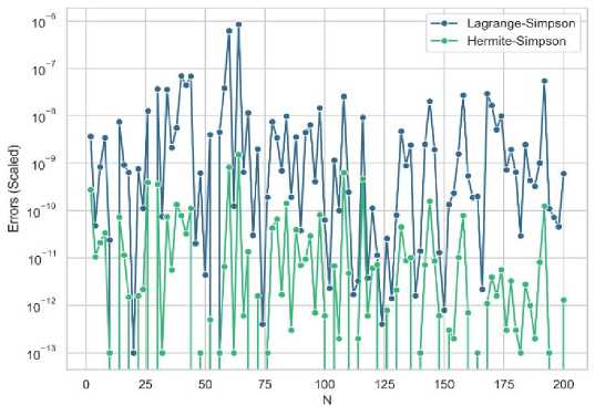
(a)   erf(2)

The volume flow rate ^ R 5 (1 — x )   2nx dx in a smooth circular pipe with radius R = 0.2

The normal distribution  1— P e a^2n: 0

m2

dx with standard deviation o' = 5 and a mean u = 10.

(d)

The moment of normal forces .^^f®2 sin2(6')de on a Block-Type Hand Brake with a maximum pressure on the shoe Pa = 27.4 psi, sin^a) J1i                                                                        1                          u face width b = 1.25 in, radius r = 6 in, a = 10, 01 = 8.13°, 02 = 98.13°, and ва = в- — 02

Fig. 1. The figures (a) through (d) show error analysis for various functions using generalized Simpson from Lagrange and Hermite methods. The graph's y-axis is scaled using a logarithmic scale to present the data effectively.

Fig. 1 shows that in various functions, generalized Simpson from Hermite exhibits lower error rates. However, this is not universally applicable. In uncommon cases, Lagrange shows lower error than Hermite (see Fig. 2). This anomaly can be attributed to the error margins of Lagrange method. This level of inaccuracy in certain scenarios, can paradoxically lead to more accurate results when dealing with higher-order polynomials (e.g., x4,x5,......,xn) or complex functions. The error introduced by Lagrange’s method may manifest as a positive error. Incorporating this error into the calculated area may enhance the overall accuracy of the method, resulting in a more precise estimate.

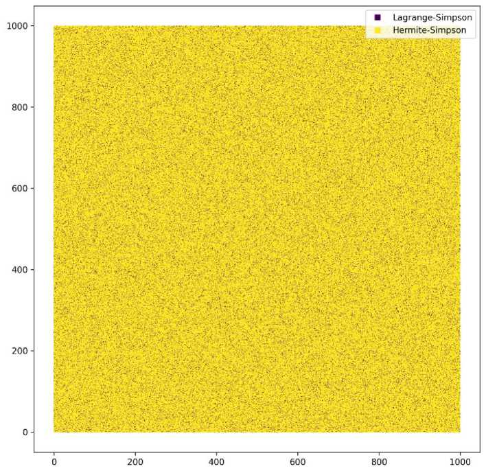
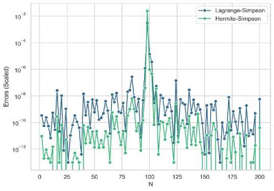
Fig. 2. The probability of Hermite Simpson and Lagrange Simpson generalizations outperforming each other across one million mesh grids.

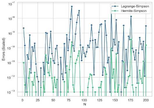
The Hermite method demonstrates a high level of stability when compared with Lagrange in generalizing Simpson's Rule. The location of c within the interval [a, b], where a, b, and c are three unevenly distributed points, has almost no significant impact on its performance. This does not hold for the Lagrange method, as the position of c significantly influences the resulting error, which decreases as we approach the midpoint of the interval (at midpoint c = 1, Hermite and Lagrange produce equivalent errors). Fig. 3 shows this behavior.

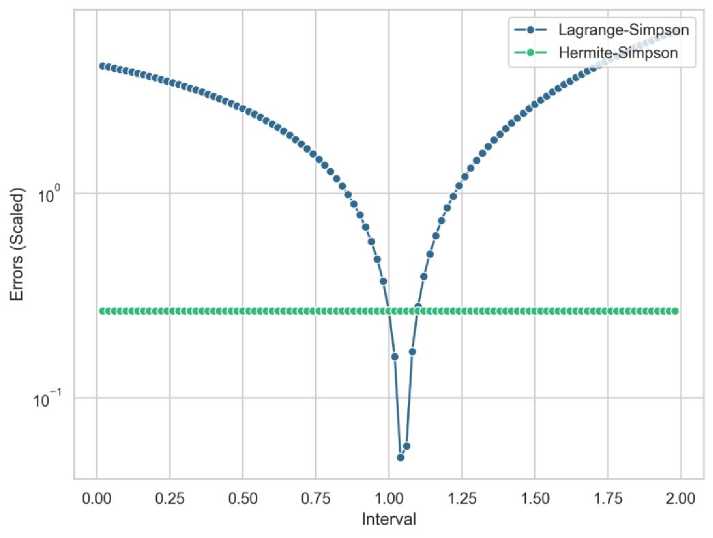
Fig. 3. Error analysis for the integration J 2 x⁴dx with varying values of c

In the example given, 198 different values for 'c' were utilized. Out of these, in 193 cases, Hermite outperformed Lagrange (97.5%), while Lagrange performed better in 4 cases (2%). Finally, in one case, their performances were found to be equal (0.05%).

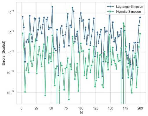
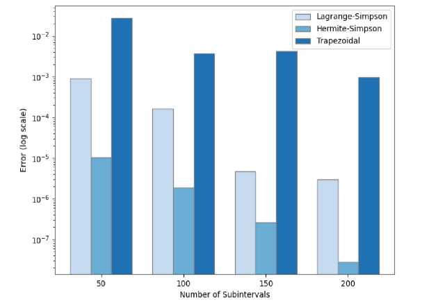
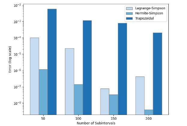
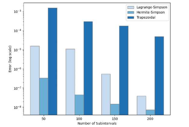
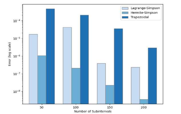
Furthermore, I employed the Trapezoidal Rule as a reference point for assessing the effectiveness of the proposed methods, given its potential adaptability to unequally spaced data. Fig. 4 shows the error analysis for each method across various functions for different subintervals (50, 100, 150, 200).

(a) I = Jo x⁴ dx

(b) ¹ = Jo '’ ■ ^dx

(c) ¹ = J o ² sⁱⁿW ^dx

(c) = J² “17 ^dx o 1+x²

Fig. 4. Performance comparison of Lagrange-Simpson, Hermite-Simpson, and Trapezoidal numerical integration methods.

Fig. 4 shows that the Hermite-Simpson method emerges as the most accurate and reliable integration method across all tested functions and subintervals. The Trapezoidal method, while simpler, exhibits the highest error terms, making it less suitable for high-accuracy requirements.

In general, the error term decreases with an increasing number of subintervals. However, the Lagrange-Simpson method presents an interesting pattern in Fig. 4b and d., where the error term increases when n = 200 for b and n = 100 for d.— indicating that this method depends on the distribution of the data used. This trend cannot be seen in Trapezoidal and Hermite-Simpson methods which both show stability.

The superior performance of the Hermite-based Simpson's Rule can be attributed to the fact that Hermite interpolation incorporates both function values and derivatives, providing a more faithful representation of the function's behavior within subintervals, particularly for functions with high curvature. While computationally more demanding, the increased accuracy offered by the Hermite generalization could be crucial in applications where even small integration errors can significantly impact results, such as in high-precision engineering design or financial modeling.

6.    Conclusions

This research presents a new generalization of Simpson’s Rule, addressing the challenge of accurately integrating functions from unequally spaced data. By employing Lagrange and Hermite interpolating polynomials, I enhance the accuracy and applicability of this widely used numerical integration technique. My findings conclusively demonstrate that the Hermite-based approach consistently surpasses the Lagrange method in terms of accuracy and stability, particularly with an increasing number of data points. However, it is more computationally costly than Lagrange because it takes into account both the function and derivative values. Although there are some cases where Lagrange outperforms Hermite, this holds true in only about 10% of cases. This anomaly can be attributed to the error margins of Lagrange method, which in some cases paradoxically lead to more accurate results. The proposed Hermite-based generalization of Simpson's Rule offers a robust and accurate solution for integrating a wide range of functions from unevenly spaced data, a problem frequently encountered in real-world applications. The rigorous comparative analysis performed, encompassing error behavior, computational cost, and sensitivity to data distribution, further strengthens the validity and practical relevance of our findings.

The enhanced accuracy achieved through the Hermite-based method translates directly into practical benefits across diverse fields reliant on precise numerical integration of unequally spaced data. For instance, in experimental data analysis, my method enables more reliable analysis of measurements with inherent uneven spacing, common due to instrument limitations or experimental constraints. This improvement is particularly valuable in applications such as calculating work done by variable forces, estimating heat transfer in systems with fluctuating temperatures, and predicting satellite trajectories from irregularly timed observations. Future research should explore the development of adaptive algorithms based on the specific characteristics of the data. Finally, applying these new methods to multidimensional integration problems with unequally spaced data presents a promising avenue for addressing increasingly complex scientific challenges.

Limitations

The study did not cover the analysis of the error terms for Generalized Simpson’s Rule using Hermite and Lagrange interpolating polynomials. Additionally, although Theorem 2 is applicable for Simpson 3/8 Rule, there was no derivation for it.