A Comprehensive Evaluation of Spectral Unmixing Methods in Hyperspectral Imaging

Author: Archana Chaudhari, Samrudhi S. Wath, Tushar P. Zanke, Stuti N. Jagtap, Snehashish S. Mulgir
Journal: International Journal of Image, Graphics and Signal Processing @ijigsp
Article in issue: 1 vol.17, 2025.
Free access
This study explores hyperspectral image classification, particularly focusing on spectral unmixing techniques applied to the widely used "PaviaU" dataset. Nine distinct endmembers, representing materials such as Water, Trees, and Shadows, serve as the foundation for our investigation. Introducing a novel linear regression model meticulously tailored for hyperspectral image reconstruction, we aim to address the complexities inherent in such datasets. Our approach leverages a fusion of non-negative least squares (NNLS) and a sum-to-one constraint, employing the Sequential Least Squares Quadratic Programming (SLSQP) method to seek optimal coefficients. Through rigorous experimentation and analysis, our model achieves a mean reconstruction error of 1152.318. The efficacy of our approach lies in its seamless integration of NNLS and SLSQP, customizing a solution to the intricate nuances of hyperspectral data. By significantly reducing reconstruction errors, our method represents a substantial advancement in spectral unmixing techniques. Furthermore, this study produces nine abundance maps for each endmember using least squares with constraints, lasso, and averaging the squared differences between observed and reconstructed spectra for pixels with nonzero class labels to determine reconstruction error. Emphasizing the importance of abundance maps and reconstruction errors, we compare the results obtained through our proposed spectral unmixing methods with those of alternative approaches. This comprehensive analysis not only sheds light on the performance superiority of our proposed methods but also provides valuable insights for practitioners and researchers working with hyperspectral imaging data. By offering enhanced accuracy and efficiency in spectral unmixing, our approach holds significant promise for applications ranging from environmental monitoring to precision agriculture and beyond.
Hyperspectral Images (HSI), Hyperspectral Unmixing (HU), Mean Reconstruction Error (MRE), Endmember Determination (ED)
Short address: https://sciup.org/15019651
IDR: 15019651 | DOI: 10.5815/ijigsp.2025.01.05
Text of the scientific article A Comprehensive Evaluation of Spectral Unmixing Methods in Hyperspectral Imaging
Hyperspectral imaging stands as a burgeoning tool across diverse research domains, offering an unparalleled depth of insight into the electromagnetic spectrum. Unlike its multispectral counterpart, hyperspectral imaging captures and processes information from numerous narrow and contiguous spectral bands, providing rich data for each pixel within an image. This detailed spectral information enables the discernment of unique material characteristics, crucial for a multitude of applications.
Central to the analysis of hyperspectral imagery is the conversion of each pixel into its constituent elements, a process known as Spectral Unmixing. Spectral Unmixing endeavors to disentangle the complex spectral signatures of mixed pixels, identifying and quantifying the contributions of different materials within remotely sensed images. The accurate extraction of endmember abundances, therefore, holds paramount importance across various fields including agriculture, geology, environmental monitoring, remote sensing, and defense.
Despite its significance, spectral unmixing poses formidable challenges due to the intricate interactions of materials and the inherent complexity of mixed spectral signatures. This paper addresses these challenges through the development and evaluation of a comprehensive methodology for spectral unmixing in hyperspectral imagery. By exploring five distinct unmixing techniques, each with its unique strengths and characteristics, this research aims to significantly advance the field.
The fundamental Least Squares method, for instance, minimizes the disparity between observed and estimated spectra, providing a foundational approach. Incorporating constraints such as sum-to-one enhances the physical interpretability of abundance fractions, while enforcing non-negativity aids in accurately separating materials, particularly with non-negative spectral signatures. Furthermore, combining sum-to-one and non-negativity constraints refines abundance maps, rendering them suitable for intricate scenes with mixed materials.
The introduction of LASSO introduces sparsity in abundance fractions, proving effective in scenarios where only a subset of endmembers significantly contributes. Through extensive experimentation and comparisons with ground truth labels, this research endeavors to elucidate the most effective techniques for accurate spectral unmixing in diverse real-world scenarios.
By advancing the methodologies for spectral unmixing in hyperspectral imagery, this research not only contributes to the theoretical understanding of the field but also holds profound practical implications. Enhanced accuracy in spectral unmixing has the potential to revolutionize various applications including land cover classification, mineral exploration, vegetation analysis, and anomaly detection, thereby shaping the landscape of environmental monitoring and beyond.
2. Literature Review
Using a synergistic approach, the paper uses both Random Forest and Deep Learning algorithms for hyperspectral image classification. The results of the study indicate that merging these strategies effectively leads to better classification accuracy[1]. Using a variety of methods, including CNN, SAM, PCA, and others, the study uses hyperspectral image analysis for early detection and classification of plant diseases and stress. The research examines efficient techniques and algorithms and presents results that show hyperspectral imaging can be used to detect problems with plant health early on[2].To classify crops, the research uses hyperspectral remote sensing and integrates various techniques and algorithms, including NDVI, CNN, MNDW, and SWIR. Results of the study show that for the corn and soya classes from Indian Pines, an overall accuracy of between 95.97% and 99.35% was attained[3]. An enhanced technique for satellite image analysis based on the Normalized Difference Vegetation Index (NDVI) is presented in this research. The false colour composite of the identified items is created using various NDVI threshold settings, The simulation's findings demonstrate how effective the NDVI is in identifying the visible area's surface features, which is crucial for municipal planning and administration[4].To enhance the precision and overall performance of hyperspectral image classification, this paper develops a feature extraction technique that combines PCA and LBP. To optimize the kernel extreme learning machine's (KELM) parameters, an optimization technique with global search capacity is used. The outcomes of the comparison experiment demonstrate that, for small samples, the PLG-KELM performs better in terms of generalization and can achieve higher classification accuracy[5].This study proposes a novel pixel-pair approach to ensure that the CNN benefit can be truly provided by greatly increasing such a number. It is anticipated that the suggested technique, which uses deep CNN to learn pixel-pair characteristics, will be more discriminative. Results from experiments using multiple hyperspectral image data sets show that the suggested approach can outperform the traditional deep learning-based approach in terms of classification performance [6]. To handle spectral variability, the paper presents a Hyperspectral Unmixing Network that makes use of a Modified Scaled and a Perturbed Linear Mixing Model. The technique improves the accuracy of hyperspectral unmixing by utilizing sophisticated algorithms such as SGA, N-FINDR, FCLS, and others, providing a new way to manage spectral variability in remote sensing applications [7].To select a band from high-dimensional data, this paper uses information entropy based on the 3D Discrete Cosine Transform. After that, a Support Vector Machine (SVM) is used to classify the chosen bands. This method produces high accuracy rates, roughly 84.61% (Indian Pines), 92.83% (Pavia University), and 94.14% (Salinas dataset). When compared to alternative band selection techniques, the suggested method shows a discernible improvement in overall classification accuracy, especially when 20 to 50 are selected[8]. The purpose of this paper is to compare the methods for extracting spatial information using the non-linear edge-preserving filter and PCA for hyperspectral classification. Following reduction bands from both techniques, Non-Linear SVM is used for classification. A varied number of bands, such as 5, 10, 15, and 25, extracted using the extraction techniques, are used to test the suggested approach. The algorithm's resilience in comparison to the other two methods is demonstrated by the university of Pavia data set's overall accuracy, average accuracy, and kappa coefficient, which are 95.87, 97.33, and 96.42, respectively[9]. The current research finds a unique strategy to picture classification by combining the image's albedo intrinsic component on principal components and factor analysis acquired through dimensionality reduction. The findings are categorized using the Support Vector Machine classifier[10].
3. Overviewof Methods 3.1 Linear Least Squares (LLS):
Linear Least Squares, often abbreviated as LLS, is a mathematical optimization technique used in regression analysis. It aims to find the linear relationship between a set of independent variables (predictors) and a dependent variable (the target) by minimizing the sum of squared differences between the observed and predicted values. In other words, it seeks to fit a linear model that best explains the relationship between the variables. First, we Load the hyperspectral data cube (HSI) containing spectral information for each pixel. Load the endmembers, which are reference spectral signatures for pure materials present in the scene. Flatten the HSI into a 2D matrix, where each row corresponds to a pixel, and each column corresponds to a spectral band. Ensure that all pixel values are non-negative. Least Squares Estimation: Formulate a linear equation for each pixel, expressing the observed spectrum as a linear combination of endmember spectra. Use the least squares method to solve these equations for the abundance fractions (coefficients). Optimize the solution by incorporating the inverse of the covariance matrix of endmembers. This minimizes the least squares error and improves estimation accuracy. Calculate the mean reconstruction error that is coming out to be 118783.181, which quantifies the quality of the unmixing results.
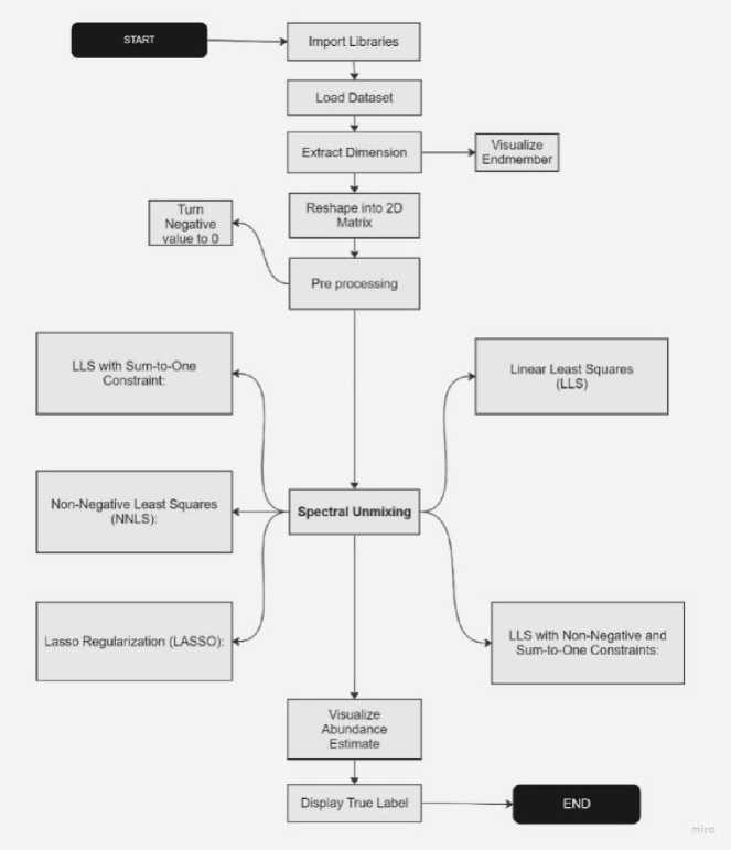
Fig. 1. Flowchart of the proposed method
Mathematically, LLS minimizes the following objective function as Eq. 1, minp∑ "=1(yi - Po - Р1Хц-⋯-fipx-tp) (1)
where:
-
• Yi is the observed value of the dependent variable for observation I.
-
• β0, β1,β2,…,βp are the coefficients to be estimated.
-
• xi1, xi2,…,xip are the values of the independent variables for observation I.
-
• n is the number of observations.
-
• p is the number of predictors.
-
3.2 LLS with Sum-to-One Constraint:
LLS finds the values of the coefficients β0, β1,β2,…,βp that minimize the sum of squared differences, resulting in the best-fitting linear model.
LLS with a sum-to-one constraint is a variation of the LLS technique. In addition to estimating abundance fractions, it enforces the constraint that these fractions must sum to one. This constraint is applicable in scenarios where the coefficients should represent proportions or weights that add up to unity.
Data Preparation: Similar to LLS, load HSI and endmembers.
Constraint Addition:Introduced an additional constraint that the estimated abundance fractions must sum to one.
Used optimization methods to solve the constrained linear system.
Calculated the mean reconstruction error which is 160049.931 to assess the accuracy of the unmixing, considering the sum-to-one constraint.
LLS with a sum-to-one constraint is a variant of LLS where an additional constraint is imposed on the coefficients. In this case, the coefficientsβ 0 , β 1 ,β 2 ,…,β p are required to sum to one as Eq. 2,
∑ pj= β j =1 (2)
This constraint is often used in applications where the coefficients represent proportions or weights that should add up to one, such as portfolio optimization or market share allocation.
-
3.3 Non-Negative Least Squares (NNLS):
Non-Negative Least Squares (NNLS) is a spectral unmixing method that extends LLS by imposing the constraint that all abundance fractions must be non-negative. This constraint is particularly useful when negative values for abundance fractions are not physically meaningful.
The NNLS can be elaborated as follows in Eq. 3. Let Y is given a set of observed hyper spectral imaging data (where each column represents a spectral signature of a pixel) and a set of end members β (where each column represents a spectral signature of an end member), and X is the abundance factor minx ‖Y- px ‖ 2f (3)
subject to the constraint X>=0
To solve this problem, various optimization techniques can be used, such as sequential quadratic programming (SQP), interior-point methods, or projected gradient descent, which iteratively updates the abundance fractions X while enforcing the non-negativity constraints until convergence is achieved.
Data Preparation: Similar to LLS, load HSI and endmembers.
Non-Negativity Constraint: Enforce the non-negativity constraint on the abundance fractions to ensure that all fractions are non-negative.
Used optimization techniques to solve the constrained linear system with non-negativity constraints.
Mean Reconstruction Error: 569339.291
In NNLS, it is required that all coefficients βj be non-negative as Eq. 4,
β j ≥ 0 for all j=0,1,2, … ,p (4)
This constraint is particularly useful when we want to ensure that the coefficients remain non-negative, which is often the case in applications like signal processing or where negative values do not make sense in the context of the problem.
-
3.4 Lasso Regularization (LASSO):
Lasso, which stands for Least Absolute Shrinkage and Selection Operator, is a regularization technique used in linear regression to prevent overfitting and select a subset of relevant features. In addition to minimizing the sum of squared differences between observed and predicted values (similar to LLS), Lasso adds a penalty term to the objective function:
Data Preparation: Load the endmembers and flatten the HSI.
For each pixel, apply Lasso regression to estimate the abundance fractions.
Lasso introduces a penalty term to the optimization problem that promotes sparsity by shrinking some coefficients to zero.
Mean Reconstruction Error: 570530.294
Mathematically, Lasso minimizes the following objective function as Eq. 5,
Minimize∑n i =1 ( yi - β 0 - β 1 xi 1 - β 2 xi 2 -…- βp xip )2+ λ ∑ j =1 p ∣ βj ∣
where:
-
• yi, β0, β1, xi1, xi2, ……, xip, n, and p have the same meanings as in LLS.
-
• βj are the coefficients to be estimated.
• λ is the regularization parameter, which controls the strength of the penalty term.
4. Proposed Method
The penalty term λ ∑p j =1 ∣ βj ∣ encourages some of the coefficients to become exactly zero, effectively selecting a subset of predictors and simplifying the model. This feature selection property of Lasso is useful in high-dimensional data where not all predictors are relevant.
Linear Least Squares with Non-Negative and Sum-to-One Constraints is our approach that combines two constraints in the context of linear regression. It builds upon the traditional LLS method but adds the requirement that both the coefficients be non-negative and that they sum to one. This approach is often applied in scenarios where you want to ensure that the estimated coefficients have specific characteristics.


Define Function Constraints
+ for Minimisation --------► Definition for Sum
Process to one
Define bound for optimization
Error Calculation Iterate over pixels
, , «------ Update Theta Я-----Spectral Unmixing abundance
Fig. 2. Proposed Method Flowchart
In our proposed model, we developed a linear regression approach tailored for hyperspectral image reconstruction. Leveraging a combination of non-negative least squares (NNLS) and an optimization strategy employing the Sequential Least Squares Quadratic Programming (SLSQP) method, our model aims to discover coefficients that effectively capture the intricate relationships between input features and observed hyperspectral data.For each pixel in the image, the model utilizes the NNLS method to obtain an initial coefficient estimate while enforcing non-negativity constraints. Subsequently, a refinement step takes place through the SLSQP optimization algorithm, where constraints are imposed to ensure that the sum of coefficients equals 1, reflecting a proportional relationship, and bounds are set to maintain non-negativity. This meticulous optimization process is performed under the condition that the corresponding pixel label is not equal to 0. This will significantly reduce reconstruction errors, there by advancing spectral unmixing.
The resulting coefficients, represented by the matrix thetaD, encapsulate the learned relationships and are employed to generate estimated values (y_estD). The mean absolute difference between the original hyperspectral data (HSI_flat) and the reconstructed values serves as a metric for the model's performance. In the case of our proposed model, the mean reconstruction error is reported as 1152.318. The efficacy of our approach lies in its ability to integrate non-negativity constraints, leveraging NNLS, and further optimizing the coefficients with SLSQP, thus offering a solution tailored to the characteristics of hyperspectral data and contributing to a significant reduction in the mean reconstruction error.
The Sequential Least Squares Quadratic Programming (SLSQP) algorithm aims to minimize a nonlinear objective function subject to nonlinear equality and inequality constraints. Mathematically it can be illustrated as Eq. 6
Minimize f ( x )
subject to:
ct ( x )≤0 for i =1,2,3,… m
ℎ 'j ( X )=0 for i =1,2,3,… n
Where: x is the vector of decision variables, f(x) is the objective function to be minimized, C^ (x) are the inequality constraint functions. ℎ j (x) are the equality constraint functions, m is the number of inequality constraints and n is the number of equality constraints.
The use of SLSQP to solve NNLS can be mathematically expressed as below;
Let's denote:
-
• X as the matrix of coefficients for all pixels in the hyperspectral image, where each column represents the coefficient vector for a pixel.
-
• Y as the matrix of observed hyperspectral data, where each column represents the spectral signature of a pixel.
-
• β as the matrix of endmembers used for reconstruction, where each column represents the spectral signature of
an endmember.
-
• n as the vector of constraints that enforce the sum of coefficients to be equal to 1.
-
• a and b as vectors representing lower and upper bounds on the coefficients to maintain non-negativity.
-
• L as the vector of labels for each pixel, indicating whether the corresponding pixel label is not equal to 0.
Then mathematical representation of the objective function is as Eq. 7
minx ‖ У - px ‖ 2f (7)
Subject to the constrains of
-
• Non Negative Constraint Xnnls ≥0
-
• cTX =1, this ensures that the sum of coefficients for each pixel equals 1, reflecting a proportional relationship.
-
• Bounds of non-negativity a ≤ X ≤ b , This imposes lower (a) and upper (b) bounds on the coefficients (X) to maintain non-negativity.
-
• Condition of pixel label L ≠0
In other words, LLS with Non-Negative and Sum-to-One Constraints minimizes the following objective function as Eq. 8, minimize∑ni=1(yi-β0-β1xi1-β2 xi2 -…-βp xip)2 (8)
Subject to the constraints: βj ≥0 for all j =0,1,2,…, ∑p j =0 βj =1 where:
• yi is the observed value of the dependent variable for observation i.
• β0, β1,β2,…,βp are the coefficients to be estimated.
• xi1, xi2,…, xip are the values of the independent variables for observation i.
• n is the number of observations.
• p is the number of predictors.
5. Result and Discussion
5.1 Dataset Description5.2 Performance Metrices
In our exploration of Spectral Unmixing, two key performance metrics stand out—mean reconstruction error and analysis of generated abundance map. Our meticulously tailored model yields a remarkably low mean reconstruction error of 1152.318. This figure encapsulates the average discrepancy between the observed and reconstructed spectra across the hyperspectral dataset, indicating the precision with which the model captures and reconstructs the complex spectral information inherent in the imagery. Simultaneously, our research underscores its technical prowess in the analysis of abundance maps. The generation of nine abundance maps for each distinct endmember—representing materials such as Water, Trees, and Shadows—utilizes the least squares method with constraints. These abundance maps provide a spatially explicit representation of the distribution and prevalence of materials within the hyperspectral scene. Rigorous analysis involves quantifying the squared differences between observed and reconstructed spectra specifically for pixels with nonzero class labels, thereby contributing to a comprehensive understanding of the model's performance in capturing the spectral signatures of various materials.
5.3 Experiment
In this approach, LLS with Non-Negative and Sum-to-One Constraints simultaneously finds the values of the coefficientsβ0, β1, β2 ,…, βp that minimize the sum of squared differences while ensuring that all coefficients are non-negative and that they sum to one. This means that the resulting linear model not only fits the data well but also adheres to the constraints specified.
The "Pavia University" hyperspectral dataset provides a detailed representation of an area within the University of Pavia in Italy using hyperspectral imaging. The dataset encompasses spatial, spectral, and class information, allowing for various remote sensing and image analysis applications. Here's an explanation of the dataset components:
HSI (Hyperspectral Image): The hyperspectral image captures information in 103 spectral bands, collected by the ROSIS sensor. The data is organized in a three-dimensional cube format, with dimensions of 300x200x103. Each pixel in the 300x200 grid corresponds to a specific location in the scene, and the 103 spectral bands provide continuous spectral information for each pixel. The ROSIS sensor captures data across a broad range of wavelengths, allowing for rich spectral characterization of materials present in the scene.
Spatial Resolution: The spatial resolution of the hyperspectral image is 1.3 meters. This means that each pixel represents an area of 1.3 meters by 1.3 meters on the ground. The high spatial resolution enables the identification of smaller objects and features within the scene.
Classes and Ground Truth: The hyperspectral image is annotated with class labels to indicate the materials or land cover types present in the scene. The dataset contains nine distinct classes, each representing a specific type of material or land cover. The class labels are provided in a separate file called "PaviaU_ground_truth.mat". Only pixels with nonzero class labels are considered in the analysis, indicating that only areas with meaningful content are included in the dataset.The "Pavia University" dataset is valuable for tasks such as land cover classification, material identification, and environmental monitoring. The dataset is combination of spectral, spatial, and class information makes it suitable for various applications in remote sensing, geospatial analysis, and machine learning.
The dataset consists of spectral signatures of 9 end members, each of them corresponding to a certain material. The spectral signatures are a unique pattern of electromagnetic radiation, typically in the form of reflected or emitted light, across different wavelengths in the electromagnetic spectrum associated with a specific material or substance. Each material interacts with light in a characteristic way, leading to a distinctive spectral signature.
Endmembers spectral signatures of Pavia University HSI
Spectral bands
Fig. 3. Spectral Signature of Endmembers
In Fig 3, the endmember and their reflectance values can be seen. The endmembers are water, trees, Asphalt, Selfblocking bricks, bitumen tiles, shadows, meadows and Bare soil. In order to Visualize the image, the 50th band is printed in Fig. 4.
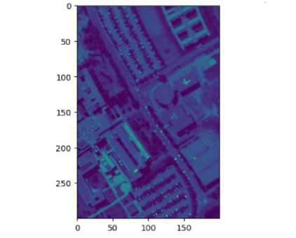
Fig. 4. 50th Band of Pavia University Dataset
The first spectral unmixing method used is least square method. The results of the method can be seen in Fig 5. The 9 abundance maps utilizing the least square method can be seen.
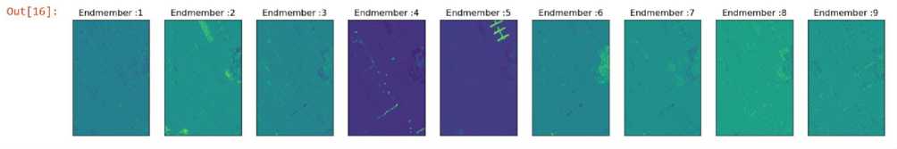
Fig. 5. Abundance Map of Least Square
Based on the method we created the mean reconstruction error for least square method is 118783.181. Next sum-to-one constraint is being imposed to the least square method. The 9 abundance maps utilizing these constraints can be seen in Fig 6. The mean reconstruction error for this method is 160049.931.
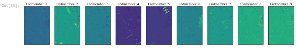
Fig. 6. Abundance Map of Least Square Imposing Sum to One Constraints
In the next spectral unmixing method non-negative constraints are being imposed on the entries of zero. The 9 abundance maps utilizing these constraints can be seen in Fig 7. The mean reconstruction error for this method is 569339.291.
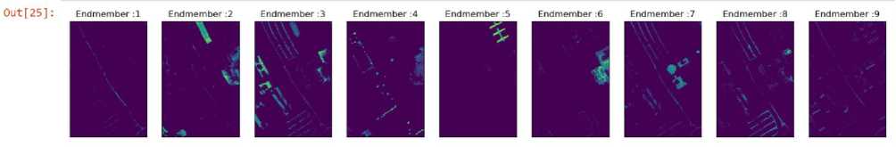
Fig. 7. Abundance Map of Least Square Imposing Non-Negative Constraints
The next method used is LASSO or Least Absolute Shrinkage and Selection Operator. The results of this method can be seen in Fig 8. The mean reconstruction error for LASSO is 570530.294.
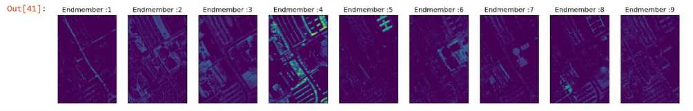
Fig. 8. Abundance Map of Lasso
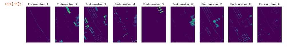
Fig. 9. Abundance Map of Least Square Imposing Sum to One and Non-Negative Constraints (Proposed Method)
The proposed method combines the sum to zero and non-negative least square methods. This in turn gives a better mean reconstruction error than other unmixing methods that are being used. The mean reconstruction error for the proposed method is 1152.318.
Table 1. Comparative analysis of Spectral unmixing methods
|
Spectral Unmixing Method Used |
Mean Reconstruction Error |
|
Least square method |
118783.181 |
|
Least square sum to one |
160049.931 |
|
Least square imposing non-negative |
569339.291 |
|
LASSO |
570530.294 |
|
Least square imposing sum to one and nonnegative Constraint (Proposed Method) |
1152.318 |
From Table 1, The results showcase the comparative performance of different spectral unmixing methods in our research. The Least Square method demonstrated a mean reconstruction error of 118,783.181, and the imposition of a sum-to-one constraint increased the error to 160,049.931. Furthermore, introducing non-negativity constraints resulted in a significantly higher error of 569,339.291. Lasso regression showed a comparable error of 570,530.294. Inour proposed method, integrating both sum-to-one and non-negativity constraints, delivered exceptional results with a substantially lower mean reconstruction error of 1,152.318. This underscores the efficacy of our tailored approach, leveraging a combination of NNLS and SLSQP optimization, to capture intricate spectral relationships and significantly enhance spectral unmixing accuracy for hyperspectral data analysis in our research.
True labels of the pixels of the Pavia University ground
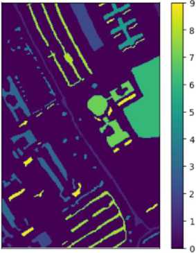
Fig. 10. Ground Truth Label
Fig 10. Present grount truth of pavia university, stored in the file "PaviaU_ground_truth.mat," provides annotations for the hyperspectral image. Each pixel in the hyperspectral image is associated with a class label, indicating the type of material or land cover present at that location. The ground truth contains a matrix or array where each entry corresponds to the class label of the corresponding pixel in the hyperspectral image.
6. Conclusions
In conclusion, our study on hyperspectral image classification for buildings and vegetation, with a specific focus on spectral unmixing, has yielded valuable insights into the efficacy of diverse methods. Using the "PaviaU" dataset with nine endmembers corresponding to distinct materials, we explored five spectral unmixing techniques: Least squares, least squares with sum-to-one constraint, least squares with non-negativity constraint, Least squares with both constraints, and LASSO. The derivation of abundance maps and computation of reconstruction errors allowed a comprehensive comparison of these methods, highlighting their individual strengths and limitations. One noteworthy outcome was the proposed method, employing Least squares with both non-negativity and sum-to-one constraints on the entries, which demonstrated promising results. The comparative analysis, with a focus on abundance maps and reconstruction errors, provided valuable insights into the practical implications of spectral unmixing techniques. The addition of class data from the dataset highlighted the practical applicability of our suggested method and further supported our conclusions. By providing a sophisticated understanding of the effects of spectral unmixing approaches on the precise delineation of urban and vegetated areas, this research advances the field of hyperspectral image categorization.
References A Comprehensive Evaluation of Spectral Unmixing Methods in Hyperspectral Imaging
- J. V. Rissati, P. C. Molina, and C. S. Anjos, “Hyperspectral Image Classification Using Random Forest and Deep Learning Algorithms,” in 2020 IEEE Latin American GRSS & ISPRS Remote Sensing Conference (LAGIRS), IEEE, Mar. 2020, pp. 132–132. doi: 10.1109/LAGIRS48042.2020.9165588.
- A. Lowe, N. Harrison, and A. P. French, “Hyperspectral image analysis techniques for the detection and classification of the early onset of plant disease and stress,” Plant Methods, vol. 13, no. 1, p. 80, Dec. 2017, doi: 10.1186/s13007-017-0233-z.
- L. Agilandeeswari, M. Prabukumar, V. Radhesyam, K. L. N. B. Phaneendra, and A. Farhan, “Crop Classification for Agricultural Applications in Hyperspectral Remote Sensing Images,” Applied Sciences, vol. 12, no. 3, p. 1670, Feb. 2022, doi: 10.3390/app12031670.
- M. Sharma, P. Bangotra, A. S. Gautam, and S. Gautam, “Sensitivity of normalized difference vegetation index (NDVI) to land surface temperature, soil moisture and precipitation over district Gautam Buddh Nagar, UP, India,” Stochastic Environmental Research and Risk Assessment, vol. 36, no. 6, pp. 1779–1789, Jun. 2022, doi: 10.1007/s00477-021-02066-1.
- H. Chen, F. Miao, Y. Chen, Y. Xiong, and T. Chen, “A Hyperspectral Image Classification Method Using Multifeature Vectors and Optimized KELM,” IEEE J Sel Top Appl Earth Obs Remote Sens, vol. 14, pp. 2781–2795, 2021, doi: 10.1109/JSTARS.2021.3059451.
- W. Li, G. Wu, F. Zhang, and Q. Du, “Hyperspectral Image Classification Using Deep Pixel-Pair Features,” IEEE Transactions on Geoscience and Remote Sensing, vol. 55, no. 2, pp. 844–853, Feb. 2017, doi: 10.1109/TGRS.2016.2616355.
- Y. Cheng, L. Zhao, S. Chen, and X. Li, “Hyperspectral Unmixing Network Accounting for Spectral Variability Based on a Modified Scaled and a Perturbed Linear Mixing Model,” Remote Sens (Basel), vol. 15, no. 15, p. 3890, Aug. 2023, doi: 10.3390/rs15153890.
- S. S. Sawant and P. Manoharan, “Unsupervised band selection based on weighted information entropy and 3D discrete cosine transform for hyperspectral image classification,” Int J Remote Sens, vol. 41, no. 10, pp. 3948–3969, May 2020, doi: 10.1080/01431161.2019.1711242.
- S. Dasi, D. Peeka, R. B. Mohammed, and B. L. N. Phaneendra Kumar, “Hyperspectral Image Classification using Machine Learning Approaches,” in 2020 4th International Conference on Intelligent Computing and Control Systems (ICICCS), IEEE, May 2020, pp. 444–448. doi: 10.1109/ICICCS48265.2020.9120945.
- L. N. P. Boggavarapu and P. Manoharan, “Classification of Hyper Spectral Remote Sensing Imagery Using Intrinsic Parameter Estimation,” 2020, pp. 852–862. doi: 10.1007/978-3-030-16660-1_83.
