A Connected Domain Analysis Based Color Localization Method and Its Implementation in Embedded Robot System

Published Online August 2011 in MECS

In many computer vision systems, color recognition always proves to be a significant means of acquiring target or environment information [1]. As a typical characteristic of visual objects, color information can be used to locate targets independently [2][3]. However, like almost all the low-level image features, color feature is also interfered greatly by noise. Although plenty of methods have been proposed, complicated filtering algorithms yield high requirement for hardware computational capability and a common embedded processor could barely meet [4]. Especially in terms of embedded systems, besides image processing, the processor also needs to take charge of other tasks such as movement scheduling. When a control algorithm is relatively sophisticated, system resources will soon be exhausted and result in an unpredictable system failure. Hoping to avoid the complexity, we intend to adopt a simple and efficient approach on the premise of a proper positioning accuracy. In general, most classic denoise techniques can be ascribed to some sort of mask-based transformation sliding over the whole frame, which would involve all the pixels repeatedly hence inducing large amount of computation. At this point, a basic motive is to find a way of locating target without particular denoise filtering.

To begin with, it is indispensable to analyze the distribution feature of image noise. Considering the general situation, employing Gaussian model to describe noise distribution is a common manner. Moreover, the output of color recognition is companied with a binarization process. When the binarization process is applied with Gaussian model, it will pose a polarized probability distribution function [5]:

P o         , z = 0

P ( z ) = 1 P        , z = 1

0 ( actually no )

That is to say, the original Gaussian model will transform to a certain salt-and-pepper noise model. On that basis, if make an assumption that the probability of noise occurrence for each pixel is independent, the probability of consecutive noise occurrence can be ignored:

N lim П P,= 0 ,0 < P,< 1       (2)

N ^^

i = 1

Following the discussion, we can develop a conclusion that a connected domain with only few pixels should be regarded to be noise, and hence by counting the pixels within regarded target areas and excluding the fewer ones, noise pixels would be suppressed notably. Furthermore, while calculating the centroid, pixel-counting is also needed; therefore both procedures can be merged without introducing extra computation.

After briefing several basic concepts above, the proposed method is summarized as follow: First, find a proper threshold from differential image for color recognition. Second, binarize the image according to this threshold. Then, labeling the image and calculate the size of each connected domain. The following verifying process will remove most noise pixels, and in the meantime, prepare necessary parameters for subsequent step. Finally, compute the centroid of each color domain coordinates and mark them on the display.

• II.    Proposed Method

The entire algorithm is comprised of three main steps shown as below: color recognition, connected domain computation, as well as positioning and marking.

• A.    Color recognition

Color recognition is a typical classification problem. That is to say, according to some certain standards, we divide the whole color set into several subsets and each subset is defined as a color. For now, we often employ the term “color space” to describe the abstract mathematical model suggesting that colors can be represented as tuples of numbers, typically as as three or four values or color components, such as the most used RGB color space. By checking the scope of each component, a color can be classified into predefined subsets.

Yet different color space models possess a variety of features. The RGB color space is influenced by luminance tremendously [6]. Table I. shows that little change in luminance (I) would bring on certain change in RGB components.

TABLE I. RGB versus HSI

R	G	B	H	S	I
40	40	220	120	60	100
36	36	198	120	60	90
32	32	176	120	60	80

Actually, human eyes will recognize all the three color as dark green even they boast obvious difference mathematically. Therefore choosing an appropriate color space is the first thing to fix. Alike the HSI color space, YUV color space also separate the luminance from other components. Yet, the implementation in YUV color space is relative complicated [7], thus our adoption of HSI color space here.

As we know, in HSI color space, sole Hue component is able to represent different color types individually. Nevertheless, when the Saturation component is lesser, validity of the Hue component would decrease, hence categorizing a color with at least both Hue and Saturation components is plausible. What is noteworthy is the conversion from RGB to HSI is a nonlinear floating point operation; the normalized formula is given below.

Normalize the raw RGB data:

R r =--------

R + G + B g = R + G + B              (3)

b =--- B---

R + G + B

Calculate each component:

0 = cos

• ^{1    [(} r - g ⁾⁺⁽ r - ^{b )]}

7 ⁽ r - g ^{) 2 +(} r - ^b X g - b )

0 h e [ 0, n ] ,for b <  g 2 n - 0 h e [ n ,2 n ] ,for b >  g s = 1 - 3 • min ( r, g, b ) s e [ 0,1 ] i = ( R + G + B ) / ( 3 • 255 ) i e [ 0,1 ]

Range conversion:

H = h Х 180/ n

S = s x 100                        (5)

I = i x 255

If applying these formulas to each pixel, definitely it should exert a heavy load to the system hardware. To the embedded system whose resources are limited, this would pose an impossible task, especially for the real-time processing. An optional way to resolve the problem is importing a lookup table (LUT) for the fast conversion. Creating the LUT is rather simple and direct: generating a 3-D array whose indexes correspond to the three RGB components, each cell comprises pre-calculated HSI components. Such as (refer to Table I.):

LUT [40] [40] [220]. H = 120

LUT [40] [40] [220]. S = 60

LUT [40] [40] [220]. I = 100

However, creating LUT according to the original 256 gray-levels consumes large amount of memory, which encourage us to use less gray-level. Considering another fact that we choose a 16bpp LCD in the hardware system, following the 16bpp format, also known as RGB565 format, would be a wise choice, simply because there is no need to add in an extra conversion between LUT accessing and image display.

I ^R I ^G I I 15                1110                  5 4                0

Figure 1. RGB565 format.

In RGB565, the Red and Blue components are represented by 5-bit binaries (32 gray-levels), while the Green component is represented by a 6-bit binary (64 gray-levels). Conversion from standard 256 gray-level (8-bit length) to these formats could be reached through integer division or logical shift. The later operation is preferred because of slightly higher efficiency, since logical instructions often use less time to get the final result. But we should note that both integer division and logical shift will omit the fraction part of quotient, which raises higher conversion error. Table II. demonstrates the integer conversion error between 256 gray-level and 32 gray-level, which is similar to other bit-lengths.

TABLE II.      I nteger C onversion E rror

raw graylevel	convert to 5-bit length	restore to 8-bit length	error
128	16 (16)	128	0
132	16 (16.5)	128	4
135	16 (16.875)	128	7
136	17 (17)	136	0

For the last row of the table, “135” is the most closed value to “136”; rather than the 5-bit gray-level “16”, it should be converted to “17” to minimize the conversion error variance. So we need an adjustment to the dividend as to obtain a rounded value. Equation (6) defines the half correction

*   1 + 1 ^{7 - b}

I = 2 8 b = ( I + 2 <<  (6 — ^b )) >>  (⁸ — b ) (6)

, where I is the original 256-level grayscale, I ^* is the rounded objective grayscale, b means the desirable bit length. For the example given above, 8-bit gray-level “135”, it would be:

l = 5 for 5 - bit grayscale

I * = (135 + (2 <<  1)) >>  3 = 139 >>  3 = 17    ⁽⁷⁾

To successfully classify a color, the next problem is how to ascertain a suitable range for each component, or to say upper and lower bound. Hoping to enhance the adaptability, a thresholding method based on frame difference (FD) is affiliated to this section. Since the system is designed to track the motion of color target, classical FD method [8] could be used to roughly locate the region of interest (ROI). By examining the occurrence probability of ROI pixels, we can obtain a fitting range for binarization. The following flowchart could help to understand the technique.

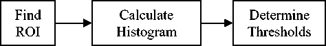
Figure 2. Thresholding flowchart for color recognition

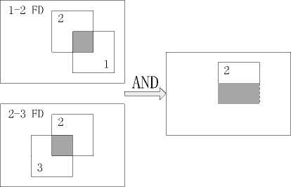
Figure 3. Using FD to find ROI.

As our interest is to find an available color region within the motion target, therefore no need to wholly fulfill the method proposed in Ref. [8] which includes a gray-level gradient calculation. Directly compute the two FD images with logical AND would meet our requirement. In Fig. 3, the upper white rectangle region enclosed by solid line is supposed to be our ROI. Color distribution within that area could be utilized to calibrate our threshold for color recognition processing. Take the gray-level image for instance; assume the typical histogram of ROI to be:

I                            Gray-level

I I I I I                  I I x

0                 к, I k2             255

Figure 4. typical histogram of ROI

Since most pixels within ROI concentrate around a solo intensity point (“I” in this example), what we need to do is find k ₁ and k ₂ to separate the axis into three classes. Otsu in his article Ref. [9] suggested a well-known method for multi-thresholding. Considering the three classes to be C 0 for [ 1, • • , k 1 ] , C 1 for [ k 1 + 1, • • , k ₂ ] and C ₂ for [ k ₂, • , L ] , the number of pixels at gray-level i is denoted by n _i and the total number of all the pixels is donated by N = n 1 + n ₂ + + n _L , the probability distribution would be:

n ^L

P i = N    , P i ^ ^{0 and} ^ P i = ^{1      (8)}

i = 1

The class occurrence probabilities are given by

® k = ^P ( ^C k ) = ^ P i , ^k = ⁰¹ , ^{2 and} ^ ® k = ^{1 (9)}

i e C_k                 k = 0

Mean levels of each class are

M k = X i ■ P (HCk )< E i ■ ^i-i e C k           i e C k ®^k

Class variance is given by

_Ofc ² = ^i-M k ) 2 P ( i\C_t ) =^-M k ) ² ■ p^ k  её,               -ёё.         ™ k

The total mean level of ROI and total variance are

L

Mk =^ i ■ Pl i=1

L

.2 =^(i-MT )2 Pi i =1

And the most important three criteria are respectively defined as

σσσ

λ = _{σ 2} , κ = _{σ 2} , η = ^B ₂          (13)

σW     σW     σT where

22 σW = ∑ωk ⋅σk k2=0                        (14)

σ B 2 = ∑ ω k ⋅ ( µ k - µ T ) 2

k = 0

Given that σ _W ² is based on the class variance, a second-order statistics, while σ _B ² is base the first-order statistics, mean level, and all these three criteria are equivalent, η is chosen to evaluate the satisfaction of thresholds due to the simpler computational complexity. Besides, σ _T ² is a constant value for each ROI, therefore by maximizing the criterion of between-class variance:

σ _B ² ( k ₁ ^* , k ₂ ^* ) = max σ _B ² ( k ₁, k ₂ )        (15)

1 ≤ k ₁ <  k ₂ ≤ 255

**

, we can get a set of fitting thresholds k ₁ and k ₂ .

If apply this method to the Hue and Saturation components of pixels within ROI, surely we can get the upper and lower bound for color recognition. Taking into consideration the fact that most factual targets seldom change their surface color, we can even put the thresholding route ahead of all the procedures as initialization. In this manner, we don’t have to change the thresholds frequently on behalf of system efficiency. The final routine could be summarized as:

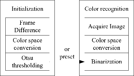
Figure 5. Full flowchart of color recognition.

• B.    Connected domain computation

The first scan is made by lines to fill an equivalence table, which depicts the starting point and end point of each line segment in the raw image, i.e. handling the horizontal connectivity. Structure of the equivalence table is:

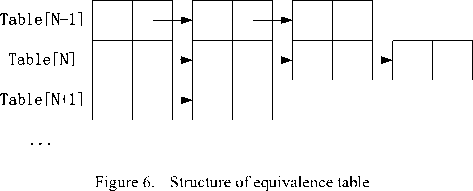
In this table each node of the linked list stands for a line segment. The second scan is made against this table. By checking the connectivity of line segments from two neighboring lines, it can be decided whether to create a new domain or merge two existing one. When the whole table is parsed, the searching is over and all the domains are found. Principle pseudo code is given below:

cur_cursor=table[i].entry a:

pre_cursor=table[i-1].entry

b:

if ( pre_cursor == null ){ area=new area area.next_node=cur_cursor

} else{ if ( pre_cursor ∈ N8 ( cur_cursor ) ){ if ( cur_cursor.area_head != null ){ if( cur_cursor.area_head != pre_cursor.area_head ) merge( cur_area , pre_area )

} else{ pre_area.next_node=cur_cursor

loop b if ( cur_cursor.area_head == null ){ area=new area;

area.next_node=cur_cursor

loop a

An example is given to illustrate the whole procedure:

0	1	1	1	1	1	1
1	1	0	1	1	0	1
0	0	1	1	0	0	0
1	1	1	0	0	1	1
0	0	0	1	1	0	0

1
2		3	4
	5
6			7
		8

Figure 7. Result of the line scan

1st line:

pre_cursor is null and cur_cursor points to line segment [1,6,6,0], i.e. [start, end, length, line index]; so create a new area A and attach the line segment to it:

2nd line:

pre_cursor points to "1" and cur_cursor points to "2"; they are 8-connected and "2" hasn't been linked to any area; so attach it to area A , which "1" belongs to:

SH2ZH2]

pre_cursor points to "1" and cur_cursor points to "3"; they are connected and "3" hasn't been linked to any area; so attach it to A :

same thing to do when cur_cursor points to "4": (5004040®

3rd line:

pre_cursor points to "2" and cur_cursor points to "5":

pre_cursor points to "3" and cur_cursor points to "5"; a little different here because "5" has already been linked to A and share the same area with "3", so nothing is done until the next line.

4th line:

pre_cursor points to "5" and cur_cursor points to "6":

<5004040404040

pre_cursor points to "5" and cur_cursor points to "7"; "7" isn't connected with any line segment (here we refer to "5") in the 3^rd line; so create a area B for it:

(0404044004040 ®0

5th line:

pre_cursor points to "6" and cur_cursor points to "8":

pre_cursor points to "7" and cur_cursor points to "8"; they are connected but belong to different area, so merge B into A :

structure is employed here, which reduces operations in adding nodes and releasing memory.

• C.    Positioning and Marking

The main purpose of color locating is to obtain target coordinates and mark them. As discussed in the introduction, if pixels of a connected domain are too few, it’s reasonable to regard it as a pseudo target. Coordinates can be calculated by the formula below:

N

0 x.

_x = J^1

N                     (16)

N

0 y-

= 1

, where x and y represent the horizontal and vertical coordinates of each pixel in one same domain, N is count of pixels. To highlight a valid target, drawing a rectangle box on the raw image would be all right, that is to ascertain the upper and lower bounds for both directions.

When in implementation, necessary parameters could be computed in the meantime of linking line segments and merging areas. For instance, while linking line segment "6" to area A , Table III. exemplifies the parameter updating procedure:

TABLE III. U pdating P arameters

	Before			After
	A		“6”	A
left	0	=	0	0
right	6	>	2	6
top	0	<	4	0
bottom	3	<	4	4
count	13	+	3	16
sigma_x	40	+	3	43
sigma_y	9	+	9	18

Like so all the required parameters could be fixed just when an area is determined, and then we can derive the final result.

III.    Experiment and Result

• A. Exper ment Platform

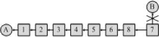
  We made our real-time experiment on an ARM system based on S3C2440, whose working frequency is 400MHz, with an external memory configuration of 64MB SDRAM working at 100MHz. Besides standard UART and Ethernet interface, a 3.5-inch LCD is also applied to display result. A common webcam (Sonix) is used as image acquisition device. Fig. 8 shows the system diagram of our experiment platform.

In this manner, we get a single connected domain marked as "A". In contrast with the method proposed in [13], based on tree structure, a simpler linked list

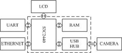
Figure 8. Hardware diagram

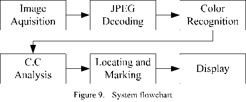
The Operating System is Linux and kernel version is 2.6.32 (V4L2 and UVC enabled). Despite that the camera can support YUYV mode, the CPU only provide a USB1.1 port, which means a compulsory MJPEG mode due to the restriction of lower bandwidth. However, performance of inexpensive webcam is often limited, whether the data are compressed won't affect the result too much. Yet extra decoding process is needed, which considerably increases the burden of our system. Flowchart of the entire system is shown as Fig. 9:

B. Results and discussion

In order to testify the effectiveness of our approach, experiments are made under the following configuration:

• •    Camera sample rate is 25FPS

• •    Sample and Display resolutions are both 320*240

• •    Preset target color is pink (Hue range from 310 to 325; Saturation is not checked)

• •    Pixel count threshold is 64 (nearly millesimal of total area)

The marking example is given below:

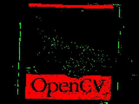
Figure 10. Binarization result

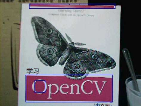
Figure 11. Marking result

After several tests, we get an output at a rate of 15 FPS on average, which meets our requirement of real-time processing. Fig. 11 illustrates a raw frame gathered from the camera and the blue rectangles marked three target color regions. Upper region is a simple connected domain, while lower regions comprise one simple connected domain (Capital letter "O") and one complex connected domain. Fig. 10 demonstrates the result of binarized image, in which red pixels indicate regarded color region. Green pixels represent noise pixels which are recognized as "pink" yet exempted by checking the count threshold. Obviously, noise pixels located within the butterfly figure and those who surround the edge of the book are inhibited effectively.

Besides above experiment using preset color threshold, we also test the adaptive threshold approach. By monitoring a ping-pong ball painted in several different colors, we get a set of threshold value. Meanwhile, this motion sequence was dumped and marked manually under the standard of maximizing the marking similarity. By checking the output of auto thresholding, we can tell whether our system could work without human interference. Since the marked image could only prove our locating approach, we draw a data table here to compares the two groups of result:

TABLE IV.     A uto and M anual C omparison

Hue	Auto thresholding		Manual Marking
Red	2	19	0	22
Green	108	125	105	129
Blue	235	247	233	252
Pink	311	328	310	325
Orange	23	36	19	34

From the table above, we can notice that our adaptive mechanism successfully realize its intension.

IV.    Conslusion

In this article, we proposed a color localization method based on connected domain analysis. It improves the efficiency by excluding additional filtering procedure. Experiments on our ARM system proved its lower computational complexity and effectiveness of noise reduction. Also, by introducing an adaptive thresholding route, it can track most targets holding relatively obvious chromatic feature without any prior knowledge or human calibration.

Admittedly, in many occasions such as targets with complex chroma composition, the thresholding approach won’t work well. Because the histogram of ROI boasts several peak values, attempting to divide all the pixels into only three classes couldn’t represent the real case. Moreover, for objects whose color may change, the system also would fail to make self-adjustment to fit the new situation. Even if we brought the adaptive thesholding into each frame, large amount of computation would still act as an insurmountable obstacle.

This system has already been applied to our robot contest, used to recognize the robot soccer. Our future research will focus on multi-feature recognition and simplifying algorithm, hoping to balance the complexity and efficiency.

Acknowledgment

The research was done thanks to financial support of the Natural Science Foundation project 2011B510017 of Education Department of Henan Province of China “Research on visual processing system of intelligent mobile robot”. The authors wish to thank all the reviewers for their valuable comments and suggestions that improved the quality of this paper.