A Face Recognition System by Embedded Hidden Markov Model and Discriminating Set Approach

Published Online July 2014 in MECS

In recent years, a large number of methods have been investigated for automatic face recognition [1][2]. Face recognition has attracted attention from the research and industrial communities with a view to achieve a “handsfree” computer controlled systems for access control, security and surveillance. As a baby one of our earliest stimuli is that of human faces. We rapidly learn to identify, characterize and eventually distinguish those who are near and dear to us. This skill stays with us throughout our lives. As humans, face recognition is an ability we accept as commonplace. It is only when we attempt to duplicate this skill in a computing system that we begin to realize the complexity of the underlying problem. Understandably, there are a multitude of differing approaches to solving this complex problem. And while much progress has-been made many challenges remain.

HMM attracts more and more attention because of its effectiveness for face recognition and facial expression recognition. The basic theory of HMM is founded by Baum at the end of 1960s.After1980s, the HMM is well known and applied in speech and printing recognition successfully [3][4]. The earliest HMM of face is built by F. Samaria in 1994 [5]. It is a one dimensional model using pixel-intensity as the observation vectors. Later, a kind of HMM with two-dimensional discrete cosine transform (2D-DCT) coefficients as observation vectors are proposed by Nefian which can be used more effectively in scale invariant systems and offer a more flexible framework for face recognition [6]. However, the image is a two-dimensional (2D) array so HMM may lose a lot of spatial information. 2D-HMM is proposed for face recognition as an enhanced version of HMM. But its application is limited due to high computational complexity and memory requirement. Then the embedded HMM (E-HMM) is introduced for face recognition by Nefian [7]. The E-HMM not only can extract main information of the2D images, but is also robust for pose and environment variation with a receivable complexity. However, the E-HMM with different parameters will generate different information expression and recognition performance, so reasonable selection of model parameters turns into an urgent problem. Aiming at this, a new face recognition algorithm is proposed based on E-HMM and Discriminating set approach. By selecting many perfect and sundry models, the sensitivity of recognition performance to E-HMM is reduced and the generalization ability of the face recognition algorithm is enhanced.

We discuss literature survey in Section II. In this section we give overview of Hidden Markov model, Embedded Hidden Markov model and Sub-Holistic Hidden Markov Model for Face Recognition. Proposed method is described in section III which consists of the discriminating set of the E-HMMs, discriminating set algorithm of E-HMMs and ensemble of E-HMM based face recognition algorithms. Experimental results are described in section IV. We discuss Experiment of face recognition based on single model and experiment of the two different sets. The recognition rates of models on different sample sets are measured in percentage (%). Section V draws a conclusion.

• II.    Literature Survey

• A.    Hidden Markov Model

Hidden Markov model is a variant of a finite state machine [8]. However, unlike finite state machines, they are not deterministic. A normal finite state machine emits a deterministic symbol in a given state. Further, it then deterministically transitions to another state. Hidden Markov models do neither deterministically, rather they both transition and emit under a probabilistic model. The hidden Markov model (HMM) is Markov model in which states are hidden. There are several types of HMM. The first distinction is made according to the nature of the probability density function used to generate all observations.

When the distribution is directly obtained through counting, HMMs are called discrete. The use of a continuous distribution, generally approximated by a mixture of Gaussian, leading to continuous HMM.

Elements of Hidden Markov Models

In order to characterize an HMM completely, following elements are needed.

N = The number of states of the model.

M =The number of distinct observation symbols per state.

T =Length of observation sequence, length of observation sequence i.e. the number of symbols observed 1, 2... N will denote the N urns respectively denote the state in which we are at time t.

V = { v 1 …v m } the discrete set of possible observation symbols.

Π = { Π i }= P (i 1 = i), the probability of being in state i at the beginning of the experiment i.e. at \=1.

A = { a ij } where a ij = P ( i t+1 =j | i t =i), the probability of being in state j at time t+1 given that we were in state i at time t.

B = { b j ( k )}, b j ( k ) = P( v k at t | i t = j), the probability of observing the symbol v k given that we are in state j.

O_t will denote the observation symbol observed at instant t.

λ = (A, B, Π) will be used as a compact notation to denote an HMM.

The image of face may be modeled using a one dimensional HMM by assigning each of these regions to a state as illustrated in Figure 1.

a11            a22

a33         a44         a55

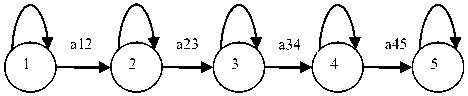
Forehead     Eyes

Nose     Mouth

Chin

Fig 1: HMM for Face recognition

In this model, the states themselves are not directly observable. What is observed are observations vectors that are statically dependent upon the state of the HMM. These vectors are obtained from L rows that are extracted sequentially from the top of each row is fixed, and the height of a face image is to its width, this HMM is restricted to fixed-size face images.

• B.    Embedded HMM

A one-dimensional HMM may be generalized, to give it the appearance of a two-dimensional structure, by allowing each state in a one-dimensional overall HMM to be an HMM. The Embedded HMM consists of a set of super states, along with a set of embedded states [9]. The super states may then be used to model two-dimensional data along one direction, with the embedded HMM modeling the data along the other direction. The elements of an embedded HMM are:

N =The number of super states, S= the set of super states, S={Si} 1≤ i ≤ N.

Π = {π, i} The initial super state distribution, where π are the probabilities of being in super state i at time zero.

A ={a,ij} = super state transition probability matrix. Where a, ij is the probability of transitioning from super state i to super state i.

Λ = super states, and the i^th super state, consisting of several embedded states, is defined as Λ = {Πi, Ai , Bi , 1 ≤ i ≤ Ns}, where Πi = {πik , 1 ≤ k ≤ N i } is the initial distribution of embedded states, N i is the number of states embedded in the i^th super state; Ai is the transition probability matrix of the embedded.

B i =state probability matrix of the i^th super state and B_t = {Ь ^ (0 _z,_y )}where b k is distribution of observation vectors in the k^th embedded state and the i^th super state. Bi is a finite mixture of the form:

bUoxy) = 2

к

CL j N( 0_xy, ^Лк ¹_к))Л<К< N^l

'7=1

Where K is the number of mixture components, each of which is described by the Gaussian probability density functions (pdf) N ( 0_xy, k^l_kj^^l_kj) with mean vector p._kj .

• C.    Sub-Holistic Hidden Markov Model for Face Recognition

Muhammad Sharif, Jamal Hussain Shah, Sajjad Mohsin, Mudassar Raza proposed a face recognition technique “Sub-Holistic Hidden Markov Model” [10]. The technique divides the face image into three logical portions. This technique, which is based on Hidden Markov Model (HMM), is then applied to these portions. The recognition process involves three steps i.e. preprocessing, template extraction and recognition. They conduct experiments on images with different resolutions of the two standard databases (YALE and ORL) and the results were analyzed on the basis of recognition time and accuracy. Sub-Holistic Hidden Markov Model for Face Recognition technique is also compared with SHPCA algorithm, which shows better recognition rates.

• III.    The Proposed Face Recognition Algorithm Based On E-Hmm And Discriminating Set

A good machine learning or pattern classification system should have a strong generalization ability, which means the ability to recognize or process the unknown things using the obtained knowledge and techniques. Therefore, generalization ability is always the ultimate problem concerned about in machine learning. Assembly learning is a new machine learning technique developed in last decades, where results of many algorithms are jointly used to solve a problem. The assembly learning cannot only improve the classification or recognition accuracy, but also obviously improve the generalization ability of the learning system. So it is regarded as one of the fourth fundamental research topics in recent years.

• A.    Discriminating SET

Here we discuss the discriminating set of the E-HMMs to improve the generalization ability. Usually, different models constructed with different parameters describe the different characteristics of the face. For example, the smaller sampling windows emphasize the local information, while the larger ones pay attention to the global information. Based on the idea of “Many could be better than all”, for the model ensemble, it is the more the better, but need to select diverse models with higher accuracy to set. Therefore, a novel face recognition algorithm is proposed based on E-HMM and discriminating set, and the scheme is shown in figure 2.

The algorithm is divided into two parts: the first part is training module, which trains n models and selects m divers models with higher accuracy for discriminating set; the second section is the assembly module, which is used to group the m selected models for face recognition.

In figure 2, M1, M2,….,Mn are models of faces with different parameters, denoted as M = (O; λ), where

O = ( o 1 , o 2 ,......, O T IP x L, A x x A y, N ₂ D -DCT)     (2)

is the feature information of the model; X = (Π ,A, Λ |Ns,Nⁱ,K ) is the structure information of the model.

Therefore, model M is determined by the above six groups of parameters.

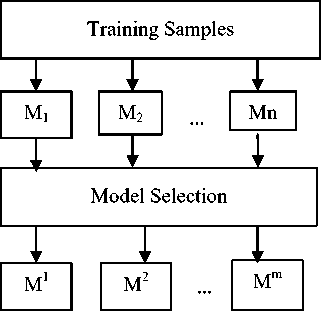
Fig 2 (a): Proposed face recognition algorithm based on EHMM and discriminating set approach training algorithm

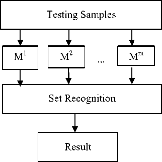
Fig 2 (b): Proposed face recognition algorithm based on EHMM and discriminating set approach recognition algorithm

• B.    The discriminating set algorithm of E-HMMs:

A discriminating set of E-HMMs is proposed in this section. Given a database with L face images, each person has l images, which consists of l1 gallery images and l2 probe images. The detailed algorithm is given as follows:

• a)    Suppose n models { M ₁ , M ₂ , . . . , M_n }are trained by the gallery images, they are used to recognize all the probe images and the corresponding recognition rates are r i ( i = 1 , 2 , . . ., n ).

• b)    Sort the n models M i ( i = 1 , 2 , . . ., n ) according to descending order of r_t as{M₁ ,М_г, ....М„,} . Let A be the set of selected models and initialized as А  {М ' }

and Z= { М1 ,М', ... М„,  }-s,m-1 models are selected by performing the following steps:

• 1.    e t is the number of faces wrongly recognized by the models in S .

• 2.    For each model M_t C Z calculate the number of the probe faces that are recognized correctly by

• 3.    S ←S ∪ И ^' , Z ←Z - M^' .

• 4.    If t < m , let t = t + 1, then go to (a), else stop and m models {M¹, M², . . . , M^m} are selected.

, (max (..,1 - । л к = { Mi ^' eZ ^{w¹ Ti ⁺w²I }} (3)

where w1 + w2 = 1, and w1 is the weight of face recognition rate, w2 is the weight of the rectifying rate.

• C.    The ensemble of E-HMM based face recognition algorithms

Using the m models {M1, M2, . . ., Mm} to recognize faces in the following method. Suppose there are H person’s images in database containing one image per person, when the probe image is input, the m selected models are used to calculate the likelihood of it belonging to each person and a likelihood matrix is resulted:

[P( o¹ | Л1 )    P ( o¹ |Д)…    p ( o¹ | ^H )

⎢ p ( o² | Я²1 )     P ( o² | Af)…     P ( o² | ^■H )⎥

⎣ ( …|․ )     ( …| ․ )…     ( …|․ )⎦

where the observation vector sequence of the probe image according to the model Mⁱ is O ⁱ ( i = 1 , 2 , . . .,m ), the E-HMM of the model Mⁱ is Z^lj ( i = 1 , 2 , . . .,m ; j =1 , 2 , . . .,H ), and P ( o^l | ^ ) ( i = 1 , 2 , . . .,m ; j = 1 , 2 , . . .,H ) is the likelihood of the probe image corresponding to the j ^th person based on the i ^th model Mⁱ. The weights of its m models for each face are wⁱ ( i = 1 , 2 , . . .,m ) and = 1.There are many ways to set weight wⁱ , such as, average weighting, namely wj =1 /m ; or setting weight according to the recognition rate:

where rⁱ is the recognition rate of the i ^th model. In order to determine the identity of a given image, the likelihood matrix P is transformed into binary matrix

Pd :

Then, the decision is made according to the following equation:

D =arg{ max, {∑^iW¹ . Pa ( O^l | ^ )}}     (7)

• IV.    Experimental Results And Analysis

Experiments are conducted to demonstrate the effectiveness of the proposed method on The Face Recognition Technology (FERET) database[18] and Georgia Tech Face Database (GTFD) [19],[20] were used. The images are at the resolution of 92×112 pixels, 8-bit gray levels. For each subject, 5 images were selected randomly as gallery images in training, the left ones are used as probe images, so sample set A is gained. Then swap the gallery and probe images, sample set B is obtained. Both A and B are utilized to determine E-HMMs of faces for assembly.

The sample sets C, D, and E are selected from database, 5 images were selected randomly as gallery images for each subject, the left 5 images are probe images. C, D and E are different from A and B. In experiment, the number of people is L = 40, the number of images for each person is l = 10, and number of gallery images is l 1 = 5, the number of probe images is l ₂ = 5. The model set is Ω = {M₁,M₂, . . .,M₂₀₀₀}, the range of parameters is set as follows: sampling window size: 2 × 2 ≤ P × L ≤ 31 × 31, sampling step: 1 × 1 ≤ Δ _x× Δ _y≤ 26 × 26, 2D-DCT coefficients: 4 ≤ N _{2 D-DCT} ≤ 24, number of pdfs: 2 ≤ N_s≤ 7, number of state: 1 ≤ Nⁱ≤ 9. In model selection module, the weight of face recognition rate is w 1 = 0 . 05, and the weight of rectifying rate is w 2 = 0 . 95.

• A.    Experiment of face recognition based on single model

In this subsection, the N models of Ω are used to recognize the sample set C, D and E, and the model recognizing each sample set optimally is denoted as MC , M_D and M_E . Model M_W was randomly selected from Ω. Model M_T is used as a reference model. The performance of each model, such as M_C , M_D and M_E , is optimal only for some certain dataset. This means that each model specializes in expressing a type of feature information rather than all features and the generalization ability of single model is not strong enough. Parameters of the above models are shown in Table I.

For the given FERET database, the recognition rates of above five models are shown in Table II, and the result indicates that the performance of each model, such as MC , M_D and M_{E ,} is optimal only for some certain dataset. This means that each model specializes in expressing a type of feature information rather than all features and the generalization ability of single model is not strong enough.

p_d ( O^l | X¹ ={¹    ifP (O< | ^)= max_k { P (O< | ^ )}

(|            0   Ot ℎ erwise

Table 1. The models and their parameters

Models	P×L	Δ x ×Δ y	N 2D-DCT	N s	K
M C	8×8	3×3	12	7	6
M D	18×18	4×4	10	4	6
M E	12×12	2×2	6	7	3
M W	31×31	24×24	6	2	2
M T	10×8	2×2	24	5	3

Table 2. The recognition rates of five models on three test samples (%)

Models	Sample set C	Sample set D	Sample Set E	Average
M C	98.4	97.7	98.6	98.23
M D	97.5	98.5	98.8	98.26
M E	97.2	98.4	98.3	97.96
M W	55.5	45.5	62.0	54.33
M T	95.5	98.5	94.0	96

• B.    Experiment of the two different sets

As previously stated, weights for sets can be set averagely or according to the recognition rate of each component model. A set of experiments are performed in order to examine the performance of E-HMM ensemble based on these two weighting methods respectively. Model sets MA and MB are selected from Ω using the method introduced in Sec. 3.2, and then, the models in each set are equally weighted to constitute Мд and Mg , while Мд and Mg are formed by unequally weighting the models. Sample sets C, D and E are recognized by these four models. The result is shown in Table III.

Table 3. Recognition results of MA and MB on three sample sets (%)

Models	Sample set C	Sample set D	Sample Set E	Average
мх	98.4	100	99	99.16
мх	98.2	99.5	98.33	98.67
MI	95.0	98.5	97.5	97
Mg	95.5	97.5	94.5	95.83

The model assembly method obtains higher recognition rate than single models, with lower variance, which shows that the proposed method leads to better and more stable recognition performance, that is to say, it can deal with new data with higher accuracy, and has strong generalization ability. This means that the proposed algorithm makes good use of recognition and error correction ability of each single model, and these component models are complemented with each other so as to improve recognition results.

• C.    Comparison experiment of face recognition algorithms

To verify the stability and generalization ability of the proposed algorithm the selective ensemble of model sets MA and MB with unequal weighting is tested respectively on dataset C, D and E. Also, we compare the our proposed algorithm with different face recognition methods such as Eigen Face [11], Fisher Face [12], Laplacianfaces [13], ML-HMM [14], MCE-HMM [15] [16], MC-HMM [17], our proposed method gives highest recognition accuracy. For all the sample sets, the recognition rate of the proposed algorithm in this paper is higher than that of the traditional algorithms based on HMM. Comparison result is summarized in Table IV.

Table 4. Comparison Results of Different Face recognition algorithms (%)

Models	Recognition rate
Proposed E-HMM	99.16
Eigenfaces	85.9
Fisherfaces	92.3
Laplacianfaces	93.2
ML-HMM	88.2
MCE-HMM	93.3
MC-HMM	97.5

• V.    Conclusion

Based on the idea of discriminating set, a multiple E-HMMs based face recognition algorithm is proposed in this paper, which solves the model selection problem in E-HMM to some extent. The experimental result shows that this algorithm achieves higher recognition rate and stronger generalization ability. That is to say, this algorithm has a stronger ability to deal with new data. Of course, the assembly of multiple E-HMMs will lead to high computational complexity. Fortunately, the new algorithm is parallel virtually, which can be used to improve the efficiency by parallel computing.