A feature selection based ensemble classification framework for software defect prediction

Автор: Ahmed Iqbal, Shabib Aftab, Israr Ullah, Muhammad Salman Bashir, Muhammad Anwaar Saeed

Журнал: International Journal of Modern Education and Computer Science @ijmecs

Статья в выпуске: 9 vol.11, 2019 года.

Бесплатный доступ

Software defect prediction is one of the emerging research areas of software engineering. The prediction of defects at early stage of development process can produce high quality software at lower cost. This research contributes by presenting a feature selection based ensemble classification framework which consists of four stages: 1) Dataset selection, 2) Feature Selection, 3) Classification, and 4) Results. The proposed framework is implemented from two dimensions, one with feature selection and second without feature selection. The performance is evaluated through various measures including: Precision, Recall, F-measure, Accuracy, MCC and ROC. 12 Cleaned publically available NASA datasets are used for experiments. The results of both the dimensions of proposed framework are compared with the other widely used classification techniques such as: “Naïve Bayes (NB), Multi-Layer Perceptron (MLP). Radial Basis Function (RBF), Support Vector Machine (SVM), K Nearest Neighbor (KNN), kStar (K*), One Rule (OneR), PART, Decision Tree (DT), and Random Forest (RF)”. Results reflect that the proposed framework outperformed other classification techniques in some of the used datasets however class imbalance issue could not be fully resolved.

Еще

Ensemble Classifier, Hybrid Classifier, Random Forest, Software Defect Prediction, Feature Selection

Короткий адрес: https://sciup.org/15016880

IDR: 15016880 | DOI: 10.5815/ijmecs.2019.09.06

Текст научной статьи A feature selection based ensemble classification framework for software defect prediction

Published Online September 2019 in MECS DOI: 10.5815/ijmecs.2019.09.06

Today, the production of high quality software at lower cost is challenging due to the large size and high complexity of required systems [1,2], [23]. However this issue can be resolved if we can predict about the particular software modules in advance, where defects are more likely to occur in future [3], [10]. The process of predicting a defective module is known as software defect prediction in which we predict the future defects at the early stages of software development life cycle (before the testing). It is considered as one of the challenging tasks of quality assurance process. Identification of defective modules at the early stage is vital as the cost of correction increases at later stages of development life cycle. Software metrics extracted from historical software data is used to predict the defective modules [29,30,31,32]. Machine learning techniques have been proved as a promising way for effective and efficient software defect prediction. These techniques are categories as 1) supervised, 2) un-supervised, and 3) hybrid. The supervised technique needs a pre-classified (training data) in order to train the classifier. During training the rules are developed which are further used to classify the unseen data (test data). In unsupervised techniques no training data is needed as these techniques use particular algorithm to identify the classes and maintain. The hybrid approach integrates the both (supervised and un-supervised). This paper proposed a feature selection based ensemble classification framework for software defect prediction. The framework is implemented from two dimensions, one with the feature selection and second without the feature selection, so that the difference of results in both dimensions can be analyzed and discussed. Each dimension further used two techniques Bagging and Boosting with Random Forest. Performance evaluation is performed from various measures such as: Precision, Recall, F-measure, Accuracy, MCC and ROC. Clean version of 12 publically available NASA datasets are used in this research including: “CM1, JM1, KC1, KC3, MC1, MC2, MW1, PC1, PC2, PC3, PC4 and PC5”. The results of the proposed framework are also compared with other widely used supervised classification techniques such as: “Naïve Bayes (NB), Multi-Layer Perceptron (MLP). Radial Basis Function (RBF), Support Vector Machine (SVM), K Nearest Neighbor (KNN), kStar (K*), One Rule (OneR), PART, Decision Tree (DT), and Random Forest (RF)”. According to results the proposed framework showed higher performance in some of the used datasets but the class imbalance problem is not fully resolved. The class imbalance issue in software defect datasets is one of the main reason of lower and biased performance of classifiers [22,23].

II. Related Work

Many researchers have used machine learning techniques to resolve the classification problems in various areas including: sentiment analysis

[11,12,13,14,15,16], network intrusion detection [17] “in press”[18],[19], rainfall prediction [20,21], and software defect prediction [10], [29] etc.. Some selected studies regarding the software defect predictions are discussed here briefly. In [10] the researchers compared the performance of various supervised machine learning techniques on software defect prediction and used 12 NASA datasets for experiments. The authors have highlighted that Accuracy and ROC did not show any reaction on class imbalance issue however Precision, Recall, F-Measure and MCC reacted on this issue with a symbol of “?” in results. In [24], the researchers used six classification techniques for software defect prediction and used the data of 27 academic projects for experiment. The used techniques are: Discriminant Analysis, Principal Component Analysis (PCA), Logistic Regression (LR), Logical Classification, Holographic Networks, and Layered Neural Networks model. Back-propagation learning technique was used to train ANN. Performance evaluation was performed by using following measures: Verification Cost, Predictive

Validity, Achieved Quality and Misclassification Rate. The results reflected that, no classification technique performed better on software defect prediction in the experiment. In [25] the researchers predicted the software defects by using SVM and compared the performance with other widely used prediction techniques including: Logistic Regression (LR), K-Nearest Neighbors (KNN), Decision Trees, Multilayer Perceptron (MLP), Bayesian Belief Networks (BBN), Radial Basis Function (RBF), Random Forest (RF), and Naïve Bayes, (NB). For experiments, NASA datasets are used including: PC1, CM1, KC1 and KC3. According to results SVM outperformed some of the other classification techniques. In [26] the researchers explored and discussed the significance of particular software metrics for the prediction of software defects. They identified the significant software metrics with the help of ANN after training with historical data. After that the extracted and shortlisted metrics were used to predict the software defects through another ANN model. The performance of the proposed technique was compared with Gaussian kernel SVM. JM1 dataset from NASA MDP repository was used for experiment. According to results the SVM performed better than ANN in binary defect classification. Researchers in [27] proposed a technique for software defect prediction which includes a novel Artificial Bee Colony (ABC) algorithm with Artificial Neural Network in order to find the optimal weights. For experiment, five publically available datasets were used from NASA MDP repository and the results reflected the higher results of proposed technique as compared to other classification techniques. In [28], the researchers introduced an approach which consists of Hybrid Genetic algorithm and Deep Neural Network. Hybrid Genetic algorithm is used for the selection and optimization of features whereas Deep Neural Network is used for classification by focusing on the selected features. The experiments were carried out on the PROMISE datasets and the results showed the higher performance of proposed approach as compared to other defect prediction techniques.

III. MAterials and Methods

This research proposes a feature selection based ensemble classification framework to predict the software defects.

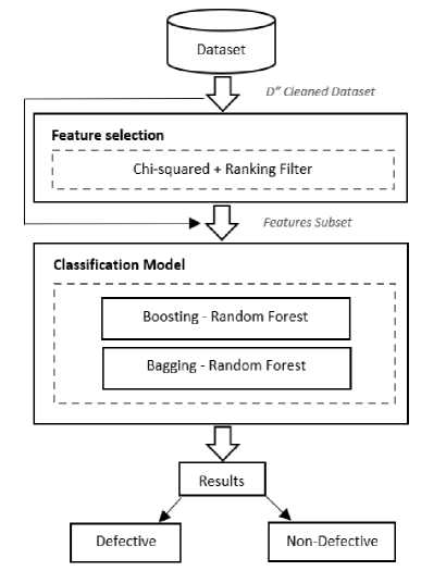
Fig.1. Proposed Classification Framework.

The proposed framework (Fig. 1) consists of four stages: 1) Dataset selection, 2) Feature Selection, 3) Classification, and 4) Results. The framework is implemented in two dimensions, in first, the feature selection stage is skipped and datasets are directly given to the ensemble classifiers however in second dimension the datasets gone through the feature selection stage. The performance of both the dimensions of proposed framework is compared with other widely used classifiers such as: “Naïve Bayes (NB), Multi-Layer Perceptron (MLP), Radial Basis Function (RBF), Support Vector Machine (SVM), K Nearest Neighbor (kNN), kStar (K*), One Rule (OneR), PART, Decision Tree (DT), and Random Forest (RF)”. All the experiments are performed in WEKA [5], which is the widely used data mining tools. It is developed in Java language at the University of Waikato, New Zealand. It is widely accepted due to its portability, General Public License and ease of use.

Dataset selection is the first stage of proposed framework. Twelve publically available cleaned NASA datasets are used in this research for experiment. The datasets include: “CM1, JM1, KC1, KC3, MC1, MC2, MW1, PC1, PC2, PC3, PC4 and PC5 (Table 2)”. Each dataset belongs to a particular NASA’s software system, and consists of various quality metrics in the form of attributes along with known output class. The output class is also known as target class and is predicted on the basis of other available attributes. The target/output class is known as dependent attribute whereas other attributes which are used to predict the dependent attribute are known as independent attributes. The datasets used in this research included dependent attribute having values either “Y” or “N”. “Y” reflects that the particular instance (module) is defective and “N” means it is nondefective. The researchers in [4] provided two versions of clean datasets: DS’ (“which included duplicate and inconsistent instances”) and D’’ (“which do not include duplicate and inconsistent instances”). Table 1 reflects the cleaning criteria implemented by [4]. We have used D’’ (Table 2) version in this research which is taken from [6]. These cleaned datasets are already used and discussed by [7,8,9,10].

Table 1. Cleaning Criteria [4]

Criterion	Data Quality Category	Explanation
1.	Identical cases	“Instances that have identical values for all metrics including class label”.
2.	Inconsistent cases	“Instances that satisfy all conditions of Case 1, but where class labels differ‘.
3.	Cases with missing values	“Instances that contain one or more missing observations”.
4.	Cases with conflicting feature values	“Instances that have 2 or more metric values that violate some referential integrity constraint. For example, LOC TOTAL is less than Commented LOC. However, Commented LOC is a subset of LOC TOTAL”.
5.	Cases with implausible values	“Instances that violate some integrity constraint. For example, value of LOC=1.1”.

Table 2. NASA Cleaned Datasets D’’ [4], [7]

Dataset	Attributes	Modules	Defective	NonDefective	Defective (%)
CM1	38	327	42	285	12.8
JM1	22	7,720	1,612	6,108	20.8
KC1	22	1,162	294	868	25.3
KC3	40	194	36	158	18.5
MC1	39	1952	36	1916	1.8
MC2	40	124	44	80	35.4
MW1	38	250	25	225	10
PC1	38	679	55	624	8.1
PC2	37	722	16	706	2.2
PC3	38	1,053	130	923	12.3
PC4	38	1,270	176	1094	13.8
PC5	39	1694	458	1236	27.0

Feature selection is the second and the most significant stage of proposed classification framework. This stage selects the optimum set of features for effective classification results. Many researchers have reported that most of the datasets only have few of the independent features which can predict the target class effectively whereas remaining features do not participate well and even can reduce the performance of classifier if not removed. We have used Chi-Square as attribute evaluator along with Ranker search method as feature selection technique.

Third stage deals with the classification with ensemble classifiers. Besides the feature selection, ensemble learning techniques have also been reported as an efficient way to improve the classification results. Bagging and Boosting are the two widely used ensemble techniques provided by Weka, which are also known as meta-learners. These techniques work by taking the base learner as argument and create a new learning algorithm by manipulating the training data. We have used Bagging and Boosting along with Random Forest as base classifier in the proposed framework.

Finally the fourth (result) stage reflects the classified modules along with the accuracy of proposed framework. The results are analyzed and discussed in detail in the next section.

IV. Results and Discussion

This section reflects the performance of proposed framework. The performance evaluation is performed in terms of various measures generated from confusion matrix (Fig. 2).

Actual Values

Defective (Y) Non-defective (N)

Defective (Y)

5 Non-defective (N) ш

TP	FP
FN	TN

Fig.2. Confusion Matrix.

A confusion matrix consists of the following parameters:

True Positive (TP): “Instances which are actually positive and also classified as positive”.

False Positive (FP): “Instances which are actually negative but classified as positive”.

False Negative (FN): “Instances which are actually positive but classified as negative”.

True Negative (TN): “Instances which are actually negative and also classified as negative”.

The performance of both the dimensions of proposed framework is evaluated through following measures: Precision, Recall, F-measure, Accuracy, MCC and ROC [22]. These measures are calculated from the parameters of confusion matrix as shown below.

Precision =--------- (TP + FP )

Re call =

(TP + FN )

Precision * Recall * 2

F-measure =-------------------

(Precision + Recall)

Accuracy =

TP + TN

TP + TN + FP + FN

AUC =

1 + TP_r - FP_r

MCC =

________ TN * TP - FN * FP ________ 4 ( FP + TP )( FN + TP )( TN + FP )(TN + FN )

The proposed framework classified the datasets in two dimensions 1) with feature selection and 2) without feature selection. In each dimension the Random Forest classifier is used with Bagging and Boosting techniques so there are total of four techniques in the proposed framework 1) Bagging-RF, 2) Boosting-RF, Feature Selection-Bagging-RF, 4) Feature-Selection-Boosting-RF. Each of the table which reflects the results also shows the score of other classification techniques such as: “Naïve Bayes (NB), Multi-Layer Perceptron (MLP). Radial Basis Function (RBF), Support Vector Machine (SVM), K Nearest Neighbor (KNN), kStar (K*), One Rule (OneR), PART, Decision Tree (DT), and Random Forest (RF)”. These results are taken from a published paper [10] in order to compare the performance of proposed framework. The paper [10] have used the same datasets (D’’) for experiments.

The results of Precision, Recall and F-Measure of each dataset for each class (Y and N) are reflected in the tables from Table 3 to Table 14. Highest scores in each class are highlighted in bold for easy identification.

Table 3. CM1 Data Results

Classifier	Class	Precision	Recall	F-Measure
NB	Y	0.1670	0.2220	0.1900
NB	N	0.9190	0.8880	0.9030
MLP	Y	0.0000	0.0000	0.0000
MLP	N	0.9040	0.9550	0.9290
RBF	Y	?	0.0000	?
RBF	N	0.9080	1.0000	0.9520
SVM	Y	?	0.0000	?
SVM	N	0.9080	1.0000	0.9520
kNN	Y	0.0670	0.1110	0.0830
kNN	N	0.9040	0.8430	0.8720
kStar	Y	0.0670	0.1110	0.0830
kStar	N	0.9040	0.8430	0.8720
OneR	Y	0.0000	0.0000	0.0000
OneR	N	0.9030	0.9440	0.9230
PART	Y	?	0.0000	?
PART	N	0.9080	1.0000	0.9520
DT	Y	0.1180	0.2220	0.1540
DT	N	0.9140	0.8310	0.8710
RF	Y	0.0000	0.0000	0.0000

	N	0.9070	0.9890	0.9460
Boost-RF	Y	0.0000	0.0000	0.0000
Boost-RF	N	0.9070	0.9890	0.9460
Bag-RF	Y	0.0000	0.0000	0.0000
Bag-RF	N	0.9070	0.9890	0.9460
Boost-RF-FS	Y	0.0000	0.0000	0.0000
Boost-RF-FS	N	0.9070	0.9890	0.9460
Bag-RF-FS	Y	0.0000	0.0000	0.0000
Bag-RF-FS	N	0.9070	0.9890	0.9460

Results of CM1 datasets are given in Table 3. The table reflects that, in Precision, NB performed better in both the classes (Y and N). In Recall, NB and DT both performed better in Y class whereas RBF, SVM and PART showed better performance in N class, and finally in F-measure, NB showed better performance in Y class whereas RBF, SVM and PART performed better in N class.

Table 4. JM1 Data Results

Classifier	Class	Precision	Recall	F-Measure
NB	Y	0.5370	0.2260	0.3180
NB	N	0.8230	0.9490	0.8820
MLP	Y	0.7650	0.0810	0.1460
MLP	N	0.8040	0.9930	0.8890
RBF	Y	0.6940	0.1040	0.1810
RBF	N	0.8070	0.9880	0.8890
SVM	Y	?	0.0000	?
SVM	N	0.7920	1.0000	0.8840
kNN	Y	0.3630	0.3340	0.3480
kNN	N	0.8290	0.8460	0.8370
kStar	Y	0.4030	0.3170	0.3550
kStar	N	0.8300	0.8760	0.8530
OneR	Y	0.3780	0.1510	0.2160
OneR	N	0.8070	0.9350	0.8660
PART	Y	0.8180	0.0190	0.0370
PART	N	0.7950	0.9990	0.8850
DT	Y	0.4960	0.2680	0.3480
DT	N	0.8280	0.9290	0.8760
RF	Y	0.5720	0.1890	0.2840
RF	N	0.8190	0.9630	0.8850
Boost-RF	Y	0.6010	0.1970	0.2970
Boost-RF	N	0.8210	0.9660	0.8870
Bag-RF	Y	0.6190	0.1780	0.2770
Bag-RF	N	0.8180	0.9710	0.8880
Boost-RF-FS	Y	0.6010	0.1970	0.2970
Boost-RF-FS	N	0.8210	0.9660	0.8870
Bag-RF-FS	Y	0.6190	0.1780	0.2770
Bag-RF-FS	N	0.8180	0.9710	0.8880

Results of JM1 datasets are reflected in Table 4. In precision, PART performed better in Y class whereas kStar performed better in N class. In Recall, kNN performed better in Y class and SVM performed better in N class. In F-measure, kStar outperformed in Y class whereas MLP and RBF outperformed in N class.

Table 5. KC1 Data Results

Classifier	Class	Precision	Recall	F-Measure
NB	Y	0.4920	0.3370	0.4000
NB	N	0.7950	0.8810	0.8360
MLP	Y	0.6470	0.2470	0.3580
MLP	N	0.7870	0.9540	0.8630
RBF	Y	0.7780	0.2360	0.3620
RBF	N	0.7890	0.9770	0.8730

SVM	Y	0.8000	0.0450	0.0850
	N	0.7530	0.9960	0.8580
kNN	Y	0.3980	0.3930	0.3950
kNN	N	0.7930	0.7960	0.7950
kStar	Y	0.4490	0.3930	0.4190
kStar	N	0.8010	0.8350	0.8170
OneR	Y	0.4440	0.1800	0.2560
OneR	N	0.7670	0.9230	0.8380
PART	Y	0.6670	0.1570	0.2550
PART	N	0.7710	0.9730	0.8610
DT	Y	0.5330	0.3600	0.4300
DT	N	0.8030	0.8920	0.8450
RF	Y	0.6150	0.3600	0.4540
RF	N	0.8080	0.9230	0.8620
Boost-RF	Y	0.5770	0.3370	0.4260
Boost-RF	N	0.8010	0.9150	0.8550
Bag-RF	Y	0.6440	0.3260	0.4330
Bag-RF	N	0.8030	0.9380	0.8650
Boost-RF-FS	Y	0.6350	0.3710	0.4680
Boost-RF-FS	N	0.8110	0.9270	0.8650
Bag-RF-FS	Y	0.6520	0.3370	0.4440
Bag-RF-FS	N	0.8050	0.9380	0.8670

Results of KC1 datasets are given in Table 5. It can be seen that in Precision, SVM outperformed in Y Class whereas RF showed better results in N Class. In Recall, kNN and kStar performed better in Y class whereas SVM showed better performance in N class, and finally, in F-measure, Boost-RF-FS performed better in Y and RBF outperform in N class.

Table 6. KC3 Data Results

Classifier	Class	Precision	Recall	F-Measure
NB	Y	0.4440	0.4000	0.4210
NB	N	0.8780	0.8960	0.8870
MLP	Y	0.5000	0.3000	0.3750
MLP	N	0.8650	0.9380	0.9000
RBF	Y	0.0000	0.0000	0.0000
RBF	N	0.8180	0.9380	0.8740
SVM	Y	?	0.0000	?
SVM	N	0.8280	1.0000	0.9060
kNN	Y	0.3330	0.4000	0.3640
kNN	N	0.8700	0.8330	0.8510
kStar	Y	0.3000	0.3000	0.3000
kStar	N	0.8540	0.8540	0.8540
OneR	Y	0.5000	0.3000	0.3750
OneR	N	0.8650	0.9380	0.9000
PART	Y	0.2500	0.1000	0.1430
PART	N	0.8330	0.9380	0.8820
DT	Y	0.3000	0.3000	0.3000
DT	N	0.8540	0.8540	0.8540
RF	Y	0.2860	0.2000	0.2350
RF	N	0.8430	0.8960	0.8690
Boost-RF	Y	0.3330	0.2000	0.2500
Boost-RF	N	0.8460	0.9170	0.8800
Bag-RF	Y	0.4000	0.2000	0.2670
Bag-RF	N	0.8490	0.9380	0.8910
Boost-RF-FS	Y	0.4170	0.5000	0.4550
Boost-RF-FS	N	0.8910	0.8540	0.8720
Bag-RF-FS	Y	0.2000	0.1000	0.1330
Bag-RF-FS	N	0.8300	0.9170	0.8710

Results of KC3 dataset is reflected in Table 6. It is reflected that in Precision, MLP and OneR showed highest performance in Y class whereas Boost-RF-FS. In Recall, Boost-RF-FS performed better in Y class and in N class, SVM outperformed the others. In F-measure,

Boost-RF-FS performed better in Y class whereas SVM performed better in N class.

Table 7. MC1 Data Results

Classifier	Class	Precision	Recall	F-Measure
NB	Y	0.1560	0.3570	0.2170
NB	N	0.9840	0.9530	0.9680
MLP	Y	?	0.0000	?
MLP	N	0.9760	1.0000	0.9880
RBF	Y	?	0.0000	?
RBF	N	0.9760	1.0000	0.9880
SVM	Y	?	0.0000	?
SVM	N	0.9760	1.0000	0.9880
kNN	Y	0.4000	0.2860	0.3330
kNN	N	0.9830	0.9900	0.9860
kStar	Y	0.2500	0.1430	0.1820
kStar	N	0.9790	0.9900	0.9840
OneR	Y	0.3330	0.1430	0.2000
OneR	N	0.9790	0.9930	0.9860
PART	Y	0.4000	0.2860	0.3330
PART	N	0.9830	0.9900	0.9860
DT	Y	?	0.0000	?
DT	N	0.9760	1.0000	0.9880
RF	Y	0.0000	0.0000	0.0000
RF	N	0.9760	0.9980	0.9870
Boost-RF	Y	0.3330	0.0710	0.1180
Boost-RF	N	0.9780	0.9970	0.9870
Bag-RF	Y	?	0.0000	?
Bag-RF	N	0.9760	1.0000	0.9880
Boost-RF-FS	Y	0.5000	0.0710	0.1250
Boost-RF-FS	N	0.9780	0.9980	0.9880
Bag-RF-FS	Y	?	0.0000	?
Bag-RF-FS	N	0.9760	1.0000	0.9880

Results of MC1 dataset are reflected in Table 7. In Precision, Boost-RF-FS showed better performance in Y class whereas NB performed better in N class. In Recall, NB performed better in Y class whereas MLP, RBF, SVM, DT, Bag-RF and Bag-RF-FS performed better in N class. In F-Measure, kNN and PART performed better in Y class whereas MLP, RBF, SVM, DT, Bag-RF, Boost-RF-FS, and Bag-RF-FS performed better in N class.

Table 8. MC2 Data Results

Classifier	Class	Precision	Recall	F-Measure
NB	Y	0.8330	0.3850	0.5260
NB	N	0.7420	0.9580	0.8360
MLP	Y	0.5000	0.5380	0.5190
MLP	N	0.7390	0.7080	0.7230
RBF	Y	0.8000	0.3080	0.4400
RBF	N	0.7190	0.9580	0.8210
SVM	Y	0.4000	0.1540	0.2220
SVM	N	0.6560	0.8750	0.7500
kNN	Y	0.6670	0.4620	0.5450
kNN	N	0.7500	0.8750	0.8080
kStar	Y	0.4000	0.3080	0.3480
kStar	N	0.6670	0.7500	0.7060
OneR	Y	0.5000	0.2310	0.3160
OneR	N	0.6770	0.8750	0.7640
PART	Y	0.7270	0.6150	0.6670
PART	N	0.8080	0.8750	0.8400
DT	Y	0.5000	0.3850	0.4350
DT	N	0.7040	0.7920	0.7450
RF	Y	0.5000	0.4620	0.4800
RF	N	0.7200	0.7500	0.7350

Boost-RF	Y	0.4550	0.3850	0.4170
	N	0.6920	0.7500	0.7200
Bag-RF	Y	0.5000	0.4620	0.4800
Bag-RF	N	0.7200	0.7500	0.7350
Boost-RF-FS	Y	0.5000	0.4620	0.4800
Boost-RF-FS	N	0.7200	0.7500	0.7350
Bag-RF-FS	Y	0.5380	0.5380	0.5380
Bag-RF-FS	N	0.7500	0.7500	0.7500

Table 8 reflects the results of MC2 dataset. It can be observed that in precision, NB performed better in Y class whereas PART performed better in N class. In Recall, PART performed better in Y class and NB and RBF performed better in N class. and finally, in F-Measure, PART showed highest results in both classes.

	N	0.9610	0.8920	0.9250
OneR	Y	0.3330	0.1000	0.1540
OneR	N	0.9550	0.9900	0.9720
PART	Y	0.3750	0.6000	0.4620
PART	N	0.9790	0.9480	0.9630
DT	Y	0.3890	0.7000	0.5000
DT	N	0.9840	0.9430	0.9630
RF	Y	0.7500	0.3000	0.4290
RF	N	0.9650	0.9950	0.9800
Boost-RF	Y	0.6000	0.3000	0.4000
Boost-RF	N	0.9650	0.9900	0.9770
Bag-RF	Y	1.0000	0.2000	0.3330
Bag-RF	N	0.9600	1.0000	0.9800
Boost-RF-FS	Y	0.6000	0.3000	0.4000
Boost-RF-FS	N	0.9650	0.9900	0.9770
Bag-RF-FS	Y	1.0000	0.2000	0.3330
Bag-RF-FS	N	0.9600	1.0000	0.9800

Table 9. MW1 Data Results

Classifier	Class	Precision	Recall	F-Measure
NB	Y	0.3330	0.6250	0.4350
NB	N	0.9500	0.8510	0.8980
MLP	Y	0.5450	0.7500	0.6320
MLP	N	0.9690	0.9250	0.9470
RBF	Y	?	0.0000	?
RBF	N	0.8930	1.0000	0.9440
SVM	Y	?	0.0000	?
SVM	N	0.8930	1.0000	0.9440
kNN	Y	0.4000	0.5000	0.4440
kNN	N	0.9380	0.9100	0.9240
kStar	Y	0.1430	0.1250	0.1330
kStar	N	0.8970	0.9100	0.9040
OneR	Y	0.5000	0.1250	0.2000
OneR	N	0.9040	0.9850	0.9430
PART	Y	0.2500	0.1250	0.1670
PART	N	0.9010	0.9550	0.9280
DT	Y	0.2500	0.1250	0.1670
DT	N	0.9010	0.9550	0.9280
RF	Y	0.3330	0.1250	0.1820
RF	N	0.9030	0.9700	0.9350
Boost-RF	Y	0.5000	0.2500	0.3330
Boost-RF	N	0.9150	0.9700	0.9420
Bag-RF	Y	0.5000	0.1250	0.2000
Bag-RF	N	0.9040	0.9850	0.9430
Boost-RF-FS	Y	0.5000	0.2500	0.3330
Boost-RF-FS	N	0.9150	0.9700	0.9420
Bag-RF-FS	Y	0.5000	0.1250	0.2000
Bag-RF-FS	N	0.9040	0.9850	0.9430

Table 9 reflects the result of MW1 dataset. It can be seen that in Precision, MLP performed better in both the classes. In Recall, MLP performed better in Y class whereas RBF and SVM performed better in in N class. In F-measure, MLP performed better in both the classes.

Table 10. PC1 Data Results

Classifier	Class	Precision	Recall	F-Measure
NB	Y	0.2800	0.7000	0.4000
NB	N	0.9830	0.9070	0.9440
MLP	Y	1.0000	0.3000	0.4620
MLP	N	0.9650	1.0000	0.9820
RBF	Y	0.3330	0.1000	0.1540
RBF	N	0.9550	0.9900	0.9720
SVM	Y	?	0.0000	?
SVM	N	0.9510	1.0000	0.9750
kNN	Y	0.2730	0.3000	0.2860
kNN	N	0.9640	0.9590	0.9610
kStar	Y	0.1250	0.3000	0.1760

Results of PC1 datasets are shown in Table 10. It can be seen that in Precision, MLP, Bag-RF, Boost-RF-FS, and Bag-RF-FS performed better in Y class whereas DT performed better in N class. In Recall, NB and DT performed better in Y class whereas MLP, SVM, Bag-RF, Boost-RF-FS, and Bag-RF-FS both performed better in N class. In F-measure, DT performed better in Y class whereas MLP performed better in N class.

Table 11. PC2 Data Results

Classifier	Class	Precision	Recall	F-Measure
NB	Y	0.0000	0.0000	0.0000
NB	N	0.9760	0.9670	0.9720
MLP	Y	0.0000	0.0000	0.0000
MLP	N	0.9770	0.9910	0.9840
RBF	Y	?	0.0000	?
RBF	N	0.9770	1.0000	0.9880
SVM	Y	?	0.0000	?
SVM	N	0.9770	1.0000	0.9880
kNN	Y	0.0000	0.0000	0.0000
kNN	N	0.9770	0.9910	0.9840
kStar	Y	0.1430	0.2000	0.1670
kStar	N	0.9810	0.9720	0.9760
OneR	Y	0.0000	0.0000	0.0000
OneR	N	0.9770	0.9950	0.9860
PART	Y	0.0000	0.0000	0.0000
PART	N	0.9770	0.9910	0.9840
DT	Y	?	0.0000	?
DT	N	0.9770	1.0000	0.9880
RF	Y	?	0.0000	?
RF	N	0.9770	1.0000	0.9880
Boost-RF	Y	?	0.0000	?
Boost-RF	N	0.9770	1.0000	0.9880
Bag-RF	Y	?	0.0000	?
Bag-RF	N	0.9770	1.0000	0.9880
Boost-RF-FS	Y	0.0000	0.0000	0.0000
Boost-RF-FS	N	0.9770	0.9950	0.9860
Bag-RF-FS	Y	?	0.0000	?
Bag-RF-FS	N	0.9770	1.0000	0.9880

Results of PC2 datasets are shown in Table 11. According to results in Precision, kStar performed well in both the classes. In Recall, kStar performed well in Y class whereas RBF, SVM, DT, RF, Boost-RF, Bag-RF, and Bag-RF-FS performed well in N class. In F-measure, kStar performed well in Y class however RBF, SVM, DT, RF, Boost-RF, Bag-RF, and Bag-RF-FS performed well in N class.

Table 12. PC3 Data Results

Classifier	Class	Precision	Recall	F-Measure
NB	Y	0.1500	0.9070	0.2570
NB	N	0.9290	0.1900	0.3160
MLP	Y	0.3460	0.2090	0.2610
MLP	N	0.8830	0.9380	0.9090
RBF	Y	?	0.0000	?
RBF	N	0.8640	1.0000	0.9270
SVM	Y	?	0.0000	?
SVM	N	0.8640	1.0000	0.9270
kNN	Y	0.4800	0.2790	0.3530
kNN	N	0.8930	0.9520	0.9220
kStar	Y	0.3130	0.2330	0.2670
kStar	N	0.8840	0.9190	0.9010
OneR	Y	0.6000	0.1400	0.2260
OneR	N	0.8790	0.9850	0.9290
PART	Y	?	0.0000	?
PART	N	0.8640	1.0000	0.9270
DT	Y	0.5000	0.2790	0.3580
DT	N	0.8940	0.9560	0.9240
RF	Y	0.6000	0.1400	0.2260
RF	N	0.8790	0.9850	0.9290
Boost-RF	Y	0.4440	0.0930	0.1540
Boost-RF	N	0.8730	0.9820	0.9240
Bag-RF	Y	0.5710	0.0930	0.1600
Bag-RF	N	0.8740	0.9890	0.9280
Boost-RF-FS	Y	0.6670	0.1400	0.2310
Boost-RF-FS	N	0.8790	0.9890	0.9310
Bag-RF-FS	Y	0.8000	0.0930	0.1670
Bag-RF-FS	N	0.8750	0.9960	0.9320

Results of PC3 dataset is reflected in Table 12. It can be seen that in Precision, Bag-RF-FS performed better in Y class however NB performed better in N class. In Recall, NB performed better in Y class whereas RBF, SVM and PART performed better in N class. In F-measure, DT performed better in Y class whereas Bag-RF-FS performed better in N class.

Table 13. PC4 Data Results

Classifier	Class	Precision	Recall	F-Measure
NB	Y	0.4860	0.3460	0.4040
NB	N	0.9010	0.9420	0.9210
MLP	Y	0.6760	0.4810	0.5620
MLP	N	0.9220	0.9640	0.9420
RBF	Y	0.6670	0.1540	0.2500
RBF	N	0.8810	0.9880	0.9310
SVM	Y	0.8180	0.1730	0.2860
SVM	N	0.8840	0.9940	0.9360
kNN	Y	0.4770	0.4040	0.4380
kNN	N	0.9080	0.9300	0.9190
kStar	Y	0.3330	0.3270	0.3300
kStar	N	0.8940	0.8970	0.8950
OneR	Y	0.6500	0.2500	0.3610
OneR	N	0.8920	0.9790	0.9330
PART	Y	0.4640	0.5000	0.4810
PART	N	0.9200	0.9090	0.9140
DT	Y	0.5150	0.6730	0.5830
DT	N	0.9460	0.9000	0.9220

RF	Y	0.7780	0.4040	0.5320
RF	N	0.9120	0.9820	0.9460
Boost-RF	Y	0.7880	0.5000	0.6120
Boost-RF	N	0.9250	0.9790	0.9510
Bag-RF	Y	0.8570	0.3460	0.4930
Bag-RF	N	0.9060	0.9910	0.9460
Boost-RF-FS	Y	0.8330	0.4810	0.6100
Boost-RF-FS	N	0.9230	0.9850	0.9530
Bag-RF-FS	Y	0.9050	0.3650	0.5210
Bag-RF-FS	N	0.9080	0.9940	0.9490

Results of PC4 datasets are shown in Table 13. It can be seen that in Precision, Bag-RF-FS performed better in Y class whereas DT performed better in N class. In Recall, DT performed better in Y class whereas SVM and Bag-RF-FS performed better in N class, and finally, In F-measure, Boosting-RF performed better in Y class whereas Boosting-RF-FS performed better in N class.

Table 14. PC5 Data Results

Classifier	Class	Precision	Recall	F-Measure
NB	Y	0.6760	0.1680	0.2690
NB	N	0.7590	0.9700	0.8520
MLP	Y	0.5600	0.2040	0.2990
MLP	N	0.7620	0.9410	0.8420
RBF	Y	0.7600	0.1390	0.2350
RBF	N	0.7560	0.9840	0.8550
SVM	Y	0.8750	0.0510	0.0970
SVM	N	0.7400	0.9970	0.8500
kNN	Y	0.5000	0.4960	0.4980
kNN	N	0.8150	0.8170	0.8160
kStar	Y	0.4390	0.4230	0.4310
kStar	N	0.7900	0.8010	0.7950
OneR	Y	0.4550	0.3360	0.3870
OneR	N	0.7760	0.8520	0.8120
PART	Y	0.6460	0.2260	0.3350
PART	N	0.7700	0.9540	0.8520
DT	Y	0.5370	0.5260	0.5310
DT	N	0.8260	0.8330	0.8300
RF	Y	0.5880	0.3650	0.4500
RF	N	0.7940	0.9060	0.8460
Boost-RF	Y	0.5880	0.3430	0.4330
Boost-RF	N	0.7900	0.9110	0.8460
Bag-RF	Y	0.6430	0.3280	0.4350
Bag-RF	N	0.7900	0.9330	0.8550
Boost-RF-FS	Y	0.5880	0.3430	0.4330
Boost-RF-FS	N	0.7900	0.9110	0.8460
Bag-RF-FS	Y	0.6430	0.3280	0.4350
Bag-RF-FS	N	0.7900	0.9330	0.8550

Results of PC5 dataset are presented in Table 14. It can be seen that in Precision, SVM performed better in Y class whereas DT performed better in N class. In Recall, DT performed better in Y class whereas SVM performed better in N Class, and finally, in F-Measure, DT performed better in Y class whereas RBF, Bagging-RF and Bagging-RF-FS outperform in N class.

Table 15. Accuracy Results

Dataset	NB	MLP	RBF	SVM	kNN	kStar	OneR	PART	DT	RF	Boost- RF	Bag-RF	Boost- RF-FS	Bag-RF-FS
CM1	82.6531	86.7347	90.8163	90.8163	77.5510	77.5510	85.7143	90.8163	77.5510	89.7959	89.7959	89.7959	89.7959	89.7959
JM1	79.8359	80.3541	80.3972	79.1883	73.9637	75.9931	77.1589	79.4905	79.1019	80.1813	80.5699	80.6131	80.5699	80.6131
KC1	74.2120	77.3639	78.7966	75.3582	69.3410	72.2063	73.3524	76.5043	75.6447	77.9370	76.7900	78.2235	78.5100	78.5100
KC3	81.0345	82.7586	77.5862	82.7586	75.8621	75.8621	82.7586	79.3103	75.8621	77.5862	79.3103	81.0345	79.3103	77.5862
MC1	93.8567	97.6109	97.6109	97.6109	97.2696	96.9283	97.2696	97.2696	97.6109	97.4403	97.4403	97.6109	97.6109	97.6109
MC2	75.6757	64.8649	72.9730	62.1622	72.9730	59.4595	64.8649	78.3784	64.8649	64.8649	62.1622	64.8649	64.8649	67.5676
MW1	82.6667	90.6667	89.3333	89.3333	86.6667	82.6667	89.3333	86.6667	86.6667	88.0000	89.3333	89.3333	89.3333	89.3333
PC1	89.7059	96.5686	94.6078	95.0980	92.6471	86.2745	94.6078	93.1373	93.1373	96.0784	95.5882	96.0784	96.0784	96.0784
PC2	94.4700	96.7742	97.6959	97.6959	96.7742	95.3917	97.2350	96.7742	97.6959	97.6959	97.6959	97.6959	97.2350	97.6959
PC3	28.7975	83.8608	86.3924	86.3924	86.0759	82.5949	87.0253	86.3924	86.3924	87.0253	86.0759	86.7089	87.3418	87.3418
PC4	86.0892	89.7638	87.4016	88.189	85.8268	81.8898	87.9265	85.3018	86.8766	90.2887	91.3386	90.2887	91.6010	90.8136
PC5	75.3937	74.2126	75.5906	74.2126	73.0315	69.8819	71.2598	75.7874	75.0000	75.9843	75.7874	76.9685	75.7874	76.9685

Table 16. ROC Area Results

Dataset	NB	MLP	RBF	SVM	kNN	kStar	OneR	PART	DT	RF	Boost-RF	Bag-RF	Boost-RF-FS	Bag-RF-FS
CM1	0.7030	0.6340	0.7020	0.5000	0.4770	0.5380	0.4720	0.6100	0.3780	0.7610	0.7650	0.7370	0.6600	0.6830
JM1	0.6630	0.7020	0.7130	0.5000	0.5910	0.5720	0.5430	0.7140	0.6710	0.7380	0.7360	0.7460	0.7360	0.7460
KC1	0.6940	0.7360	0.7130	0.5210	0.5950	0.6510	0.5510	0.6360	0.6060	0.7510	0.7510	0.7570	0.7510	0.7500
KC3	0.7690	0.7330	0.7350	0.5000	0.617	0.5280	0.6190	0.7880	0.5700	0.8070	0.7850	0.8150	0.8340	0.8670
MC1	0.8260	0.8050	0.7810	0.5000	0.6380	0.6310	0.5680	0.6840	0.5000	0.8640	0.8350	0.8470	0.8270	0.8830
MC2	0.7950	0.7530	0.7660	0.5140	0.6680	0.5100	0.5530	0.7240	0.6150	0.6460	0.6650	0.6700	0.6460	0.6570
MW1	0.7910	0.8430	0.8080	0.5000	0.7050	0.5430	0.5550	0.3140	0.3140	0.7660	0.7260	0.7420	0.7260	0.7610
PC1	0.8790	0.7790	0.8750	0.5000	0.6290	0.6730	0.5450	0.8890	0.7180	0.8580	0.8960	0.9210	0.9240	0.9100
PC2	0.7510	0.7460	0.7240	0.5000	0.4950	0.7910	0.4980	0.6230	0.5790	0.7310	0.6560	0.7740	0.4890	0.5630
PC3	0.7730	0.7960	0.7950	0.5000	0.6160	0.7490	0.5620	0.7900	0.6640	0.8550	0.8360	0.8390	0.8500	0.8410
PC4	0.8070	0.8980	0.8620	0.5830	0.6670	0.7340	0.6140	0.7760	0.8340	0.9450	0.9450	0.9530	0.9520	0.9550
PC5	0.7250	0.7510	0.7320	0.5240	0.6570	0.6290	0.5940	0.7390	0.7030	0.8050	0.7990	0.8050	0.7990	0.8050

Table 17. MCC Results

Dataset	NB	MLP	RBF	SVM	kNN	kStar	OneR	PART	DT	RF	Boost-RF	Bag-RF	Boost-RF-FS	Bag-RF-FS
CM1	0.0970	-0.0660	?	?	-0.0370	-0.037	-0.074	?	0.0410	-0.032	-0.032	-0.032	-0.032	-0.032
JM1	0.2510	0.2060	0.2150	?	0.1860	0.2120	0.1260	0.1040	0.2520	0.2440	0.2620	0.2560	0.2620	0.2560
KC1	0.2500	0.2960	0.3470	0.1510	0.1900	0.2380	0.1470	0.2390	0.2910	0.3460	0.3090	0.3440	0.3640	0.3550
KC3	0.3090	0.2950	-0.1070	?	0.2180	0.1540	0.2950	0.0560	0.1540	0.1110	0.1450	0.1850	0.3300	0.0220
MC1	0.2080	?	?	?	0.3250	0.1740	0.2060	0.3250	?	-0.006	0.1450	?	0.1820	?
MC2	0.4440	0.2430	0.3710	0.0400	0.3740	0.0620	0.1370	0.5120	0.1890	0.2160	0.1410	0.2160	0.2160	0.2880
MW1	0.3670	0.5890	?	?	0.3730	0.0380	0.2110	0.1100	0.1100	0.1500	0.3020	0.2110	0.3020	0.2110
PC1	0.4000	0.5380	0.1610	?	0.2470	0.1280	0.1610	0.4400	0.4900	0.4590	0.4050	0.4380	0.4380	0.4380
PC2	-0.0280	-0.0150	?	?	-0.0150	0.1460	-0.010	0.0150	?	?	?	?	-0.010	?
PC3	0.0880	0.1830	?	?	0.2940	0.1730	0.2450	?	0.3040	0.2450	0.1540	0.1910	0.2650	0.2460
PC4	0.3340	0.5150	0.2790	0.3420	0.3590	0.2250	0.3520	0.3960	0.5140	0.5160	0.5840	0.5070	0.5930	0.5410
PC5	0.2450	0.2160	0.2510	0.1730	0.3140	0.2270	0.2090	0.2740	0.3610	0.3220	0.3100	0.3360	0.3100	0.3360

We have considered F-measure for analysis from Table 3 to Table 14 with ‘Yes’ class. F measure is selected as it provides the average of Precision and Recall and ‘Yes’ class predicts the probability of defective modules. It has been observed from the results of F-measure that the proposed framework outperformed only in three datasets KC1, KC3 and PC4. In Accuracy (Table 15), the proposed framework performed better in four datasets including JM1, PC3, PC4, and PC5. In remaining datasets either the result is lower or equal to one or more of the other classification techniques. It has also been noted that NB, kNN, and kStar could not be able to perform better in any of the dataset. In ROC Area, the higher performance is reflected in the following datasets: CM1, JM1, KC1, KC3, MC1, PC1, and PC4 however the results in remaining datasets shows either lower or equal performance when compared to other classification techniques. It has also been observed that RBF, SVM, kNN, OneR, PART, and DT could not be able to perform better in any of the dataset. In MCC, the proposed framework showed the higher performance in following datasets: JM1, KC1, KC3 and PC4. In remaining datasets the scores are either lower or equal, as compared to other classification techniques. It has also been noted that RBF, SVM, OneR, RF, Bag-RF, and Bag-RF-FS could not be able to perform better in any of the dataset.

As discussed by [10], F- measure and MCC reacts to the issue of class imbalance however it has been observed in this study that our proposed framework could not be able to fully solve that issue either.

V. Conclusion

This research proposed and implemented a feature selection based ensemble classification framework. The proposed framework consisted of four stages including: 1) Dataset, 2) Feature Selection, 3) Classification, and 4) Results. Two different dimensions are used in the framework, one with feature selection and second without feature selection. Each dimension further used two ensemble techniques with Random Forest classifier: Bagging and Boosting. Performance of proposed framework is evaluated through Precision, Recall, F-measure, Accuracy, MCC and ROC. For experiments, 12 Cleaned publically available NASA datasets are used and the results of both the dimensions are compared with the other widely used classification techniques such as: “Naïve Bayes (NB), Multi-Layer Perceptron (MLP). Radial Basis Function (RBF), Support Vector Machine (SVM), K Nearest Neighbor (KNN), kStar (K*), One Rule (OneR), PART, Decision Tree (DT), and Random Forest (RF)”. Results showed that the proposed classification framework outperformed other classification techniques in some of the datasets however class imbalance issue could not be resolved, which is the main reason of lower and biased performance of classification techniques. It is suggested for future work that the resampling techniques should be included in proposed framework to resolve the class imbalance issue in datasets as well as to achieve higher performance.

Список литературы A feature selection based ensemble classification framework for software defect prediction

S. Huda, S. Alyahya, M. M. Ali, S. Ahmad, J. Abawajy, J. Al-Dossari, and J. Yearwood, “A Framework for Software Defect Prediction and Metric Selection,” IEEE Access, vol. 6, pp. 2844–2858, 2018.
E. Erturk and E. Akcapinar, “A comparison of some soft computing methods for software fault prediction,” Expert Syst. Appl., vol. 42, no. 4, pp. 1872–1879, 2015.
Y. Ma, G. Luo, X. Zeng, and A. Chen, “Transfer learning for crosscompany software defect prediction,” Inf. Softw. Technol., vol. 54, no. 3, Mar. 2012.
M. Shepperd, Q. Song, Z. Sun and C. Mair, “Data Quality: Some Comments on the NASA Software Defect Datasets,” IEEE Trans. Softw. Eng., vol. 39, pp. 1208–1215, 2013.
I.H. Witten and E. Frank, Data Mining: Practical Machine Learning Tools and Techniques, second ed. Morgan Kaufmann, 2005.
“NASA Defect Dataset.” [Online]. Available: https://github.com/klainfo/NASADefectDataset. [Accessed: 01-July-2019].
B. Ghotra, S. McIntosh, and A. E. Hassan, “Revisiting the impact of classification techniques on the performance of defect prediction models,” Proc. - Int. Conf. Softw. Eng., vol. 1, pp. 789–800, 2015.
G. Czibula, Z. Marian, and I. G. Czibula, “Software defect prediction using relational association rule mining,” Inf. Sci. (Ny)., vol. 264, pp. 260–278, 2014.
D. Rodriguez, I. Herraiz, R. Harrison, J. Dolado, and J. C. Riquelme, “Preliminary comparison of techniques for dealing with imbalance in software defect prediction,” in Proceedings of the 18th International Conference on Evaluation and Assessment in Software Engineering. ACM, p. 43, 2014.
A. Iqbal, S. Aftab, U. Ali, Z. Nawaz, L. Sana, M. Ahmad, and A. Husen “Performance Analysis of Machine Learning Techniques on Software Defect Prediction using NASA Datasets,” Int. J. Adv. Comput. Sci. Appl., vol. 10, no. 5, 2019.
M. Ahmad, S. Aftab, I. Ali, and N. Hameed, “Hybrid Tools and Techniques for Sentiment Analysis: A Review,” Int. J. Multidiscip. Sci. Eng., vol. 8, no. 3, 2017.
M. Ahmad, S. Aftab, and S. S. Muhammad, “Machine Learning Techniques for Sentiment Analysis: A Review,” Int. J. Multidiscip. Sci. Eng., vol. 8, no. 3, p. 27, 2017.
M. Ahmad, S. Aftab, and I. Ali, “Sentiment Analysis of Tweets using SVM,” Int. J. Comput. Appl., vol. 177, no. 5, pp. 25–29, 2017.
M. Ahmad and S. Aftab, “Analyzing the Performance of SVM for Polarity Detection with Different Datasets,” Int. J. Mod. Educ. Comput. Sci., vol. 9, no. 10, pp. 29–36, 2017.
M. Ahmad, S. Aftab, M. S. Bashir, N. Hameed, I. Ali, and Z. Nawaz, “SVM Optimization for Sentiment Analysis,” Int. J. Adv. Comput. Sci. Appl., vol. 9, no. 4, 2018.
M. Ahmad, S. Aftab, M. S. Bashir, and N. Hameed, “Sentiment Analysis using SVM: A Systematic Literature Review,” Int. J. Adv. Comput. Sci. Appl., vol. 9, no. 2, 2018.
A. Iqbal and S. Aftab, “A Feed-Forward and Pattern Recognition ANN Model for Network Intrusion Detection,” Int. J. Comput. Netw. Inf. Secur., vol. 11, no. 4, pp. 19–25, 2019.
A. Iqbal, S. Aftab, I. Ullah, M. A. Saeed, and A. Husen, “A Classification Framework to Detect DoS Attacks,” Int. J. Comput. Netw. Inf. Secur., vol. 11, no. 9, pp. 40-47, 2019.
S. Behal, K. Kumar, and M. Sachdeva, “D-FAC: A novel ϕ-Divergence based distributed DDoS defense system,” J. King Saud Univ. - Comput. Inf. Sci., 2018.
S. Aftab, M. Ahmad, N. Hameed, M. S. Bashir, I. Ali, and Z. Nawaz, “Rainfall Prediction in Lahore City using Data Mining Techniques,” Int. J. Adv. Comput. Sci. Appl., vol. 9, no. 4, 2018.
S. Aftab, M. Ahmad, N. Hameed, M. S. Bashir, I. Ali, and Z. Nawaz, “Rainfall Prediction using Data Mining Techniques: A Systematic Literature Review,” Int. J. Adv. Comput. Sci. Appl., vol. 9, no. 5, 2018.
S. Wang and X. Yao, “Using class imbalance learning for software defect prediction,” IEEE Transactions on Reliability, vol. 62, no. 2, pp. 434–443, 2013.
J. C. Riquelme, R. Ruiz, D. Rodr´ıguez, and J. Moreno, “Finding defective modules from highly unbalanced datasets,” Actas de los Talleres de las Jornadas de Ingenier´ıa del Software y Bases de Datos, vol. 2, no. 1, pp. 67–74, 2008
F. Lanubile, A. Lonigro, and G. Visaggio, “Comparing Models for Identifying Fault-Prone Software Components,” Proc. Seventh Int’l Conf. Software Eng. and Knowledge Eng., pp. 312–319, June 1995.
K. O. Elish and M. O. Elish, “Predicting defect-prone software modules using support vector machines,” J. Syst. Softw., vol. 81, no. 5, pp. 649–660, 2008.
I. Gondra, “Applying machine learning to software fault-proneness prediction,” J. Syst. Softw., vol. 81, no. 2, pp. 186–195, 2008.
O. F. Arar and K. Ayan, “Software defect prediction using cost-sensitive ¨ neural network,” Applied Soft Computing, vol. 33, pp. 263–277, 2015.
C. Manjula and L. Florence, “Deep neural network based hybrid approach for software defect prediction using software metrics,” Cluster Comput., pp. 1–17, 2018.
R. Moser, W. Pedrycz, and G. Succi, “A Comparative Analysis of the Efficiency of Change Metrics and Static Code Attributes for Defect Prediction”, In Robby, editor, ICSE, pp. 181–190. ACM, 2008.
E. Giger, M. D’Ambros, M. Pinzger, and H. C. Gall, “Method-level bug prediction,” in ESEM ’12, pp. 171–180, 2012.
S. E. S. Taba, F. Khomh, Y. Zou, A. E. Hassan, and M. Nagappan, “Predicting bugs using antipatterns,” in Proc. of the 29th Int’l Conference on Software Maintenance, pp. 270–279, 2013.
K. Herzig, S. Just, A. Rau, and A. Zeller, “Predicting defects using change genealogies,” in Software Reliability Engineering (ISSRE), 2013 IEEE 24th International Symposium on, pp. 118–127, 2013.

Еще

Статья научная