A Fully Adaptive and Hybrid Method for Image Segmentation Using Multilevel Thresholding

Author: Salima Ouadfel, Souham Meshoul
Journal: International Journal of Image, Graphics and Signal Processing(IJIGSP) @ijigsp
Article in issue: 1 vol.5, 2013.
Free access
High level tasks in image analysis and understanding are based on accurate image segmentation which can be accomplished through multilevel thresholding. In this paper, we propose a new method that aims to determine the number of thresholds as well as their values to achieve multilevel thresholding. The method is adaptive as the number of thresholds is not required as a prior knowledge but determined depending on the used image. The main feature of the method is that it combines the fast convergence of Particle Swarm Optimization (PSO) with the jumping property of simulated annealing to escape from local optima to perform a search in a space the dimensions of which represent the number of thresholds and their values. Only the maximum number of thresholds should be provided and the adopted encoding encompasses a continuous part and a discrete part that are updated through continuous and binary PSO equations. Experiments and comparative results with other multilevel thresholding methods using a number of synthetic and real test images show the efficiency of the proposed method.
Image segmentation, Multilevel thresholding, Particle swarm optimization, Simulated annealing
Short address: https://sciup.org/15012523
IDR: 15012523
Text of the scientific article A Fully Adaptive and Hybrid Method for Image Segmentation Using Multilevel Thresholding
Multilevel thresholding is an important technique that has many applications in image processing, including segmentation, clustering and object discrimination. It aims to separate the objects and the background of the image into non overlapping regions. Thresholding may require the use of one or more thresholds depending on the number of classes that should be depicted in an image. Therefore, based on this assumption, thresholding methods can be divided into two main categories namely bi-level thresholding and multi-level thresholding. In bi-level thresholding, pixels within an image are classified into two classes that consist of the object class and the background class depending on whether their values are above or below a given threshold. By extension, multilevel thresholding involves several thresholds to classify pixels into more classes. A good review of bi-level and multilevel thresholding algorithms can be found in [1].
Depending on the way to find the thresholds, both bilevel and multilevel thresholding methods can be divided into parametric and nonparametric approaches. The parametric approach is based on a statistical model of the pixel grey level distribution. Generally, a set of parameters that best fits the model is derived using least square estimation. This typically leads to nonlinear optimization problems that are computationally expensive and time-consuming [2, 3]. In the nonparametric approach, the search of the optimal thresholds is done by optimizing an objective function based on some discriminating criteria such as between class variance [4] and entropy [5].
A large number of thresholding methods have been proposed in the literature in order to perform bi-level thresholding and most of them are easily extendable to multilevel thresholding. Despite the straightforwardness of this extension process, the computational time will increase sharply when the number of thresholds is too high because of the exhaustive searching they perform [6]. This weakness makes the multilevel thresholding methods unsuitable in many applications and explains the need to use faster and robust optimization methods for multilevel thresholding problem [7]. As a consequence, several fast techniques have been proposed in the literature such as recursive algorithms [8]. Huang and Wang [9] propose a two-stage multithreshold based on Otsu’s method. Wang and Chen [10] applied an improved shuffled frog-leaping algorithm to the three dimensional Otsu thresholding. Li and Tam presented a fast iterative implementation for the minimum cross entropy thresholding method [11]. Chung and Tsai [12] proposed a fast implementation of binarization algorithm using an efficient heap and quantization based data structure. A recursive programming technique using the maximum cross entropy was proposed by Yin [13]. Shelokar et al. [14] selected the optimal threshold by minimizing the sum of the fuzzy entropies. Despite the good results of these methods, they still suffer from the problem of long processing time when the number of threshold increases, due to their iterative process.
This limitation has motivated the researchers to find new optimization methods that require moderate memory and computational resources, and yet produce good results. Therefore, metaheuristics have been used as computationally efficient alternatives to traditional multilevel thresholding methods to solve the multilevel thresholding problem. A metaheuristic is a high-level general purpose search strategy which helps exploring large search spaces in order to find good quality feasible solutions. Metaheuristics have been most generally applied to NP-Complete problems and to other combinatorial optimization problems for which a polynomial-time solution exists but is not practical. Since their apparition, metaheuristics have proven their efficiency in solving complex and intricate optimization problems arising in various fields. The most popular and used ones are the Genetic algorithm (GA) [15], Particle Swarm Optimization (PSO) [16], Differential Evolution (DE) algorithm [17], Simulated Annealing (SA) [18], Artificial Bee Colonies (ABC) Algorithm [19], Bacterial Foraging (BF) algorithm [20] … etc. Due to their capacity to escape from local optima and their ability to find good quality solutions within a reasonable time, several researchers have applied metaheuristics in multilevel thresholding context. Examples of such attempts include the use of GA algorithm [7, 21, 22, 23], DE algorithm [24, 25, 26], PSO algorithm [27, 28, 29, 30], ABC algorithm [31, 32], BFA algorithm [33]. A good review of metaheuristic algorithms for multilevel thresholding can be found in [34].
Despite the relative efficiency of most of methods in the literature to find the optimal thresholds, they all require the number of thresholds to be specified in advance. However, in many practical cases, it is difficult, even impossible to determine the exact number of thresholds without a prior knowledge. Few algorithms have been designed to automatically determine the suitable number of thresholds. Fuzzy entropy is used in [35] to select automatically the optimal number of thresholds and their location in the image histogram. Yen et al. [36] proposed a new criterion for multilevel thresholding, called Automatic Thresholding Criterion (ATC). This criterion includes a bi-level method that correlates the discrepancy between the original and thresholded image and the number of bits used to represent the segmented image [1, 36]. In this strategy, the histogram image is divided into two more sequentially up to the minimum of the cost function ATC is reached [36]. In each step the distribution with the largest variance is further dichotomized in two more distributions by applying the same bi-level thresholding. A new dichotomization process of the ATC method was proposed in [37].
Although the dichotomization techniques are fast algorithms, they are sub-optimal techniques and so they do not allow providing the optimal threshold values [7]. The GA presented in [7] determines the threshold number as well as the optimal threshold values. In their method, the wavelet transformation is used to reduce the length of the histogram and the GA algorithm optimizes the ATC criterion. Recently, Djerou et al. proposed in [38] an automatic multilevel thresholding approach, based on Binary PSO algorithm, which uses the Otsu’s criterion and the Kapur’s entropy as objective function. In [39] author adapts the intelligent water drops (IWDs) algorithm to optimize a modified Otsu’s criterion for automatic multilevel thresholding.
PSO is a population-based metaheuristic introduced by Kennedy and Eberhart in 1995 [16] as an alternative to the standard Genetic Algorithm (GA). PSO was inspired by social behavior of bird flocking or fish schooling. Each particle within a swarm searches the solution space for the best solution by changing its position with time according to its own experience, and to the experience of neighboring particles. The main advantages of PSO are its flexibility, its robustness and its inherent parallelism. It has been applied in many kinds of engineering problem widely and has proved its large capability to competing with other classical optimization algorithms [40, 41, 42, 43, 44]. However, observations reveal that the PSO suffers from a premature convergence: it converges rapidly in the early stages of the searching process, but can be trapped in a local optimum in the later stages. To overcome this drawback of diversity loss, different hybrid PSOs with others metaheuristics like SA, GA, DE have been proposed. A good and recent review of hybrid PSO can be found in [45, 46].
In this paper, we propose a new automatic multilevel thresholding technique based on PSO. The new method is able to determine both the appropriate number of thresholds and the appropriate threshold values by optimizing ATC [36]. We adopt AMT-PSOSA (Automatic Multilevel Thresholding with PSO and SA) as an acronym to the algorithm we propose in this paper. AMT-PSOSA uses a new hybrid representation to allow particles to contain different thresholds numbers within a given range defined by minimum and maximum threshold number. Particles are initialized randomly to process different cluster numbers in a specified range and the goal of each particle is to search the optimum number of thresholds and the optimum threshold values. In order to allow PSO jump out of a local optimum, SA is applied to some particles of the swarm if no improvement occurs in their best local fitness during a number of iterations. Thus, at the start of SA most worsening solutions may be accepted, but at the end only improving ones are likely to be accepted. This procedure will help PSO to jump out of a local minimum.
The rest of this paper is organized as follows: Section 2 introduces, briefly, PSO and SA algorithms. Section 3 is devoted to detailed descriptions of AMT-PSOSA. The experimental results are evaluated and discussed in section 4. Finally, conclusions are given in section 5.
-
II. Backround
-
A. Particle swarm optimization
Particle swarm optimization (PSO) is a populationbased evolutionary computation method first proposed by Kennedy and Eberhart [16]. It is inspired from the natural behavior of the individuals in a bird flock or fish school, when they search for some target (e.g., food). The PSO algorithm is initialized with a swarm of particles (called potential solutions) randomly distributed over the search area. Particles fly through the problem space by following the current optimum particle and aim to converge to the global optimum of a function attached to the problem.
Each particle i in the swarm is represented by two elements: its current position ( p i ), and its velocity ( v i ). Its movement through the search space is influenced by its personal best position pbest i it has achieved so far and the local best value lbest , obtained so far by any particle in the neighbors of the particle. When a particle takes all the population as its topological neighbors, the lbest value is a global best and is called gbest . If the problem space is D-dimensional and the swarm size is Np , at each iteration t , the particle’s new position and its velocity are updated as follows:
v j = wvT + C1 X r l ( P best - P^ ) +
-
c 2 X r 2( P gbest — P y 1 ) (1)
where i = 1,2, . . . , Np ; j = 1,2, . . . , D
The parameter w is an inertia weight [47] used in order to control the values of the velocity. The inertia weight w is equivalent to a temperature schedule in the simulated annealing algorithm and controls the influence of the previous velocity: a large value of w favors exploration, while a small value of w favors exploitation. As originally introduced in [47], w decreases linearly during the run from wmax to wmin. c1 and c2 are two constants which control the influence of the social and cognitive components such that C + c2 = 4. r and r are two random values in the range [0,1].
The main steps of PSO algorithm are presented in algorithm 1.
The particle swarm optimization approach presented above works on continuous space. However, for some optimization problems, a discrete binary representation is better for the particles than a real representation. To deal with this kind of optimization problems, Kennedy and Eberhart proposed in [48] the Binary PSO (BPSO).
Algorithm 1
Initialize all parameters
Initialize particle’s positions and velocities
Set pbest for each particle
Compute gbest repeat for each particle do
Calculate fitness value
Update pbest if improvement end
Update gbest for each particle do
Calculate particle velocity according to (1)
Update particle position according to (2)
end until maximum iterations is not attained
BPSO preserves the fundamental concept of the Real PSO algorithm and differ from it essentially in two characteristics: first, candidate solutions consists of binary strings each representing a particle’s position vector. Second, the velocity represents the probability of bit p i taking the value 1.
The position update equation is defined by:
-
'0 if r > f ( v t - 1)
P t =i j (3)
i _1 if r < f (vt-1)
with
f ( <-1) = I------(4) '' 1 + exp(-v^ )
where r is a random value with range [0, 1]. To avoid saturation of the sigmoid function in (4), the velocity can be limited in the range [- V max ,V max ].
Despite the fast convergence of PSO, it has been observed that the PSO algorithm can be trapped in a local minimum. This premature convergence occurs because particles fly to local, or near local, optimums, therefore, the balance between the exploration process (searching of the search space) and exploitation process (convergence towards the optimum) is disturbed. In order to overcome this problem, the PSO technique can be combined with some other evolutionary optimization technique to yield an even better performance [43]. In this paper, PSO algorithm is hybridized with the SA algorithm. The hybrid algorithm takes both of fast searching ability in PSO and the advantages of probability jumping property of SA. Other applications of hybrid PSO and SA algorithm can be found [49, 50, 51, 52, 53].
-
B. Simulated Annealing (SA) algorithm
The original concept of SA was proposed by American physicist Metropolis et al. [54]. It is inspired from the annealing process in metallurgy, which is a method using heat and controlled cooling of a material to increase the size of its crystals. The heat destabilizes the atoms from their first positions and wanders randomly through states of higher energy. It has observed that when the cooling is slow, it gives the atoms more chances of finding configurations with lower internal energy than the initial one.
Kirkpatrick et al. gives in [18] a mathematical model of the annealing process and uses this model for finding solutions for combinatorial optimized problems, and was the first literature to successfully utilize SA. The principle of SA is to accept solutions of worse quality than the current solution in order to escape from local optima. The probability of accepting such worst solutions is decreased during the search.
A standard SA procedure begins by generating random initial solution called current solution cs. At the initial stages, SA attempts to replace the current solution cs by random solution cs’ that is generated by making a small random change in the current solution cs . The objective function f ( cs’ ) of the new solution is calculated and the metropolis acceptance rule is then used to determine if the generated solution should be accepted or not as the new current solution. A move to the new solution cs’ is made if it improves the current solution cs that is f(cs’ ) is better than f(cs) otherwise it may be accepted with a probability that depends both on the difference between the corresponding function values f(cs) and f(cs’ ) and also on a global parameter T (called temperature) that is gradually decreased during the cooling process. In rejection case, a new solution is generated and evaluated. Typically this step is repeated until the system reaches a solution that is good enough for the problem, or until a given number of iterations is reached. The probabilistic metropolis acceptance mechanism is defined by the following
P = e^/T )
where
P : Probability for acceptance.
A E : The fitness difference between both the fitness of the new generated solution cs’ and the fitness of the current solution cs .
T : Temperature value.
The temperature T is decreases during the search process; at the beginning of the search process, the solutions with the worst fitness value are accepted with a high probability and this probability is gradually decreased at the end of the search process.
The pseudo-code of SA algorithm is given in algorithm 2.
Algorithm 2
Let cs th e current solution
Evaluate cs and store its fitness value f ( cs )
Initialize best_solution with the current solution cs
Initialize T 0 (initial temperature) and T f (final temperature)
Initialize T to T 0
while T>Tf do for a fixed number of iterations do
Generate new solution cs’ in the neighborhood of the current solution cs
Evaluate the fitness value of the new solution cs’
AE = f (cs') - f (cs)
if A E <0 then cs=cs’
( -A E / T )
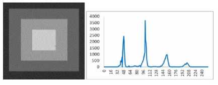
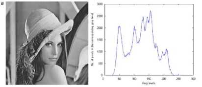
else if rand (0,1) Update best_ solution with the new generated solution cs’ end T = a* T End The SA algorithm has a strong ability to find the local optimistic result. With its jump probability, it can avoid the problem of local optimum, but its ability of finding the global optimistic result is weak. In order to improve the results of SA algorithm, it can be used with other techniques like PSO to improve the results. III. AMT-PSOSA: the proposed automatic MULTILEVEL THRESHOLDING METHOD In this section, we describe a new automatic image segmentation algorithm using multilevel thresholding based on a hybridization of PSO with SA. Given a gray level image I to be segmented into meaningful regions. Let there be L gray level values lying in the range {0,1, 2,…..,(L-1)}. For each gray level i, we associate h(i) which represents the number of pixels having the ith gray level as a value. Therefore, the probability pi of the ith gray level is defined as pi=h(i)/N L-1 where N = ^ h (i) denotes total number of pixels in i=0 the image I . Suppose image I is composed of M+1 regions. Hence, M thresholds, {t1,t2,…….,tM} are required to achieve the subdivision of the image into regions: C0 for [t0 ,...., 11 - 1] , Ci for [t 1 ,...., t2 - 1] , , Cm for [tM,...., L -1] ,such that tx < t2 — "-tM 1 — tjw ■ The thresholding problem consists in choosing the set of optimal thresholds (t*, t*,......, t* ) that maximizes an objective function f that is: J* X Z ZZAX (ti,t2,.....,1m) = argmax (f (t)) (6) where t is a potential solution in the feasible region. The aim of AMT-PSOSA algorithm is to search both the numbers of thresholds as well as the optimal threshold values using the global search capability of PSO and its fast convergence combined with the efficiency of SA to escape from local minimum. The framework of the AMT-PSOSA algorithm is given in algorithm 3 below. Algorithm 3 Initialize all parameters (listed in Table 1) for each particle Xi do Initialize particle’s position Initialize particle’s velocities stochastically Initialize pbest end Initialize gbest position and Mbest iter ← 0 while (iter < itermax) do for each particle Xi do Update particle velocity Enforce velocity bounds Update particle ‘s position Enforce position bounds Evaluate particle’s fitness Record new pbest value of the particle end Record new gbest and Mbest Select particles that are evolved by SA for each selected particle Xi do T ← T0 current_solution ← pbesti current_fitness ← f itness(current_solution) while ( T>Tf) do iterSA ← 0, // iteration of SA algorithm while (iterSA< iterSAmax) do Generate neigh_solution Evaluate neigh_solution‘s fitness if accept (neigh_solution) then current_solution ← neigh_solution end iterSA←iterSA+1 Update pbesti if improvement end t = a* t end end Update gbest position and Mbest iter ← iter + 1 end Segment the image using the optimal number of thresholds Mbest and the optimal thresholds values given by gbest. A. Particle representation Since in this paper, we have to optimize the threshold values and the number of thresholds, we have chosen to represent the particle with both real values and binary values. The real values are used to select the optimal threshold values which are updated by Real PSO algorithm. Binary values are used to select the optimal number of thresholds using the Binary PSO. The Real PSO and Binary PSO evolve in parallel contribute in the evaluation of the fitness function. In this representation, a binary mask is associated with each threshold value. The value of this mask determines whether the threshold value is used in the thresholding process or not. The initial population For a particle Xi, each probably threshold value t ( 1 = X....T ) is associated with a mask Y,, . The ij .... max ij . threshold value is taken into account if its ij corresponding mask is set to 1 that is: yy = 1 and discarded otherwise that is y^ = 0 . Therefore, for each particle, the total number of masks set to 1 gives the number of thresholds Mi encoded in it, that is: T max Mi = £ Y j=1 For a Tmax thresholds problem, the position of a particle is formulated as: X = (y 1, Yi2 max max If after initialization, it is found that no mask could be set to “1” in a particle (all threshold values are invalid), one random mask is selected and set to 1. Thus a valid particle should include at least one mask set to 1 in its position vector. Two examples of the particle structure in the proposed approach are shown on Figure 1. masks field ,—л---, [0,1,0,1,0, thresholdsvalues 12, 45, 160, 225, 225] mask field thresholdsvalues ,—л—, '----------л----------' [1,0,1,0,1, 10, 50, 100, 210, 240] Figure 1. Two examples of the particle structure in the AMT-PSOSA algorithm. In the first example, particle Xi represents 3 classes (2 thresholds), and the associated thresholds values are 45 and 225. Thresholds values 12, 160 and 250 are invalid and not used to thresholding the image. In the second example, particle Xi represents 4 classes (3 thresholds), and the associated thresholds values are 10, 100 and 240. Thresholds values 50 and 210 are invalid and not used to thresholding the image. The position of each particle is changed using the following rule: the threshold values are update using continuous PSO equations whereas the mask field is changed using equations of Binary PSO. In addition the velocity of each particle must lie within the interval [0,1]. B. Population initialization To generate the initial population of particles, we use in this paper the random generation strategy until all particles in a population are created. Each individual particle Xi of the population is initialized by randomly chosen threshold values within the range [gmin, gmax], where gmin and gmax are the minimum and the maximum gray levels in the image, respectively. tj) = gmin + rand0 * (gmax - gmJ (8 In addition, masks are , i i max randomly chosen and their values are set to “1”. C. Fitness evaluation The fitness of a particle indicates the degree of goodness of the solution it represents. In this work the fitness of a particle is computed using the cost function ACT [36]. Let M, ^ , ц , and ц be the number of thresholds encoded in a particle, the probability of the class Ci , the mean grey level of the class Ci and the total mean grey level of the image, respectively: ti —1 11 —1 ^i = 2Pj, Pi = EiPj/®t, цE j=t- j=t- where pj is the normalized probability at level j Let c2, а2 and а2 be the within-class variance, the w, BT between-class variance and the total class variance, respectively. They are given by the following expressions: M t -1 Ox M) =22' - Pi )2 Pj, i-0 j = и M2 7в = 2 ю,\ц,-ц) i=0 L-1 ат=2(j - ц)2 Pj j=0 The ACT function proposed by Yen et al. is defined as follows: F (M) = p * (Disk (M ))1/2+ (log2( M ))2 (9) The Disk(M) represents the within-class variance and is defined as: Disk (M) = c2 - 72 (M) The first term of F(M) measures the cost incurred by the discrepancy between the thresholded image and the original image. The second term measures the cost resulted from the number of bits used to represent the thresholded image. In this equation, p is a positive weighting constant and it is set to 0.8 in this study as recommended in [36]. The number of thresholds is determined by counting the number of “1” in the mask field of the particle position and the corresponding threshold values are determined accordingly. The fitness fitness (M) of a particle which encoded M thresholds is defined as: fitness (M) = —-— F(M) When the algorithm converges, the found number of thresholds M* and the corresponding found thresholds values are determined by the particle that has the maximum value of fitness function throughout the entire run. D. SA-based local search As a metaheuristic based method, PSO has a strong ability in finding the most optimistic result. Meanwhile, it can be trapped in a local optimum. SA has a strong ability in finding a local optimistic result, but its ability in finding the global optimistic result is weak [52]. Combining PSO and SA leads to the combined effect of two algorithms: the fast convergence of the PSO and its efficient global search and the efficient local search of SA and its ability to avoid local minima, which gives better results. There are many ways to combine PSO with SA, but the best one is which take advantage of probability jumping property of SA without increasing the computational cost or altering the fast convergence ability of PSO. In this paper, we apply the jump property of SA to the process of updating the local best positions of selected particles in the swarm. Indeed, it would be helpful for the best particles to jump out the local minima, and as a result, the whole swarm would move to better positions. SA algorithm is applied for a particle if it is selected with an adaptive probability Pe as in [22]. Let gbest the global best fitness of the current iteration; pbest be the average fitness value of the population and pbesti be the fitness value of the solution (particle) to be evolved. The expression of probability, Pe is given below: Pe k2 x (gbest - Pbest ) (gbest - Pbest ) k4 if Pbest, > Pbest if Pbestt < Pbest Here, values of k2 and k4 are kept equal to 0.5 [22]. This adaptive probability helps PSO to avoid getting stuck at local optimum. The value of Pe increases when the fitness of the particle is quite poor. In contrast when the fitness of the particle is a good solution, Pe will be low. SA starts with a local best solution pbest of a selected particle Xi and generates a random neighbor solution using a heuristic strategy. A valid threshold t ( γ = 1 )in Xi is chosen to undergo a perturbation operation with probability equal to 0.2. The threshold value is then modified as follows: new old ij ij gmax - gmin ) new ij gmin,gmax where tnew and told represent the new and the old threshold value. δis a random number between [-1, 1]. Thus the solution encoded by the particle is reconfigured, although the number of thresholds belonging to it remains unaltered. After the SA-based local search is completed, the gbest of the whole swarm should be updated if a solution with better quality is found during the local search. IV. Experimental results In order to assess the ability of the proposed algorithm to determine the number of thresholds and to achieve good quality image segmentation, synthetic and real images (Lena, Pepper, Baboon, Airplane, Hunter and Cameraman) have been used. Figures 2 and 3 show these test images along with their histograms. All real images are of size (512 x 512) except the Pepper image which is of size (256 x 256). Experiments have been carried out for several number of thresholds M ranging from 2 to 5. First experiments have been conducted to set the control parameters used in the AMT-PSOSA algorithm. Their values are gathered in Table 1. The quality of the thresholded image has been evaluated using the uniformity measure defined by the following equation: Figure 3. Real test images and their histograms a)Lena; b) Pepper, c)Mandril, d) Airplane, e) Hunter, f) Cameraman Figure 2. Synthetic image and its histogram. M ∑∑(gi-µj)2 U=1-2*(M) j=0 i∈Rj N*(g gmax - gmin ) Where M is the number of thresholds, Rj is the segmented region j, gi is the grey level of pixel i µj is the mean of grey levels of those pixels in segmented region j N is the total number of pixels in the given image, gmax is the maximal grey level of the pixels in the given image, gmin is the minimum grey level of the pixels in the given image, The domain of the uniformity measure is the range [0,1]. A higher value of uniformity means that the quality of the thresholded image is better. TABLE 1. PARAMETER SETTINGS FOR AMT-PSOSA ALGORITHM Parameters Values Population size (Np) 50 Maximum Inertia weight (wmax) 0.9 Minimum Inertia weight (wmin) 0.4 Maximum velocity (Vmax) +1.0 Minimum velocity (Vmin) -1.0 Cognitive coefficient (C1) 1.429 Cognitive coefficient (C2) 1.429 Maximum number of iterations (itermax ) 1000 // parameter values of SA algorithm Initial temperature (T0) 1000 Final temperature (Tf) 1 Annealing rate ( α ) 0.99 maximum number of iteration (iterSAmax) 100 TABLE 2. PARAMETER SETTINGS FOR THE GA AND DMTBPSO ALGORITHMS. Parameter set for the GA algorithm Values Population size (Np) 100 Crossover probability (Pc) 0.9 Mutation probability (Pm) 0.1 Maximum number of iterations 1000 Parameter set for the DMTBPSO algorithm Values Population size (Np) 100 р • ini 0.5 Inertia weight (w) 0.72 Maximum velocity (Vmax) 255 Cognitive coefficient (C1) 2 Cognitive coefficient (C2) 2 Maximum number of iterations 1000 To further appreciate the performance of the proposed method, experimental results from the multilevel thresholding technique based on the recently developed automatic multilevel thresholding algorithm DMTBPSO [38] and on a classical PSO and GA algorithms have been examined and compared with the proposed method AMT-PSOSA. In order to make an objective comparison, the results through an exhaustive search method are also presented. GA-based method, PSO-based method and the exhaustive search method use Otsu’s criterion as objective function defined below: M fOtsu(M)=∑ωk(µk-µ )2 k=0 In the following we will refer to them as ES-Otsu, GA-Otsu, PSO-Otsu and DMTBPSO. Parameter values of GA and DMTBPSO algorithms are presented in Table 2. We employ the best possible parameter settings recommended for DMTBPSO algorithm in [38]. PSO-Otsu is implemented using the same parameter values of AMT-PSOSA. For GA-Otsu, PSO-Otsu and ES-Otsu, the number of thresholds must be given in advance. In order to compare them with the proposed AMT-PSOSA, we must reformulate them in such a way that the number of thresholds is extracted automatically. As in [7], GA-Otsu, PSO-Otsu and ES-Otsu are executed in this paper with varying gradually the number of thresholds. The optimal threshold number, which optimizes the cost function ATC defined, is recorded. The main steps of this algorithm are given in algorithm 4 below [7]. Algorithm 4 1. M=1 2. Apply the ES-Otsu method or the GA-Otsu method or PSO-Otsu method using the number M of thresholds 3. Compute the value of the cost function F(M) by using the output optimal thresholds values 4. If F(M) is decreased, set M=M+1 and go to step 2 else go to step 5 5. Output the threshold number M* and the optimal thresholds values obtained from the corresponding multilevel thresholding method. Moreover, in order to investigate the effects of the hybridization of the PSO with SA, we have compared AMT-PSOSA with a classical PSO based multilevel thresholding method (AMT-PSO) which uses the same particle representation scheme and fitness function as the AMT-PSOSA. Table 3 summarize the obtained results for the synthetic and real images using the proposed AMT-PSOSA algorithm and the other multilevel thresholding algorithms including the optimal number of thresholds, the corresponding best ATC function value and the uniformity measure related to the synthetic image and the six real test images. Also the computing time of each algorithm is given for each image. From this table, we can draw the following conclusions: The computational time of the exhaustive search method (ES-Otsu) is very expensive and increases sharply when the number of the thresholds increases. AMT-PSO and AMT-PSOSA algorithms provide the same threshold number than GA-Otsu, PSO-Otsu and ES-Otsu algorithms, for all test images. The results of AMT-PSO and AMT-PSOSA algorithms are better than those of DMTBPSO algorithm. AMT-PSOSA is better that AMT-PSO which means that performance is greatly improved by the SA-local search procedure. In most cases, the performance of the proposed method, evaluated through the optimal threshold number M*, the cost function F(M) and the uniformity measure U, are close to those of ES-Otsu. From computation time view point, the proposed method gives a reasonable CPU time, even though the SA-local search is added. TABLE 3. COMPARISON OF PERFORMANCES FOR SYNTHETIC AND REAL TEST IMAGE Image Algorithms M* Thresholds values ATC function Uniformity CPU time Synthetic image ES-Otsu 3 74-126-176 6.353374 0.997436 9.897 GA-Otsu 3 74-126-176 6.353374 0.997436 0.987 PSO-Otsu 3 74-126-176 6.353374 0.997436 0.645 DMTBPSO 3 81-125-171 6.513393 0.997218 1.092 AMT-PSO 3 74-126-176 6.353374 0.997436 0.065 AMT-PSOSA 3 74-126-176 6.353374 0.997436 0.480 Lena ES-Otsu 4 75-114-145-180 9.948331 0.991877 5571.872 GA-Otsu 4 74-112-145-180 9.948545 0.987776 0.987 PSO-Otsu 4 74-114-145-180 9.948331 0.991877 0.468 DMTBPSO 4 78-117-150-187 10.04973 0.991598 0.428 AMT-PSO 4 73-113-146-185 9.950145 0.991750 0.062 AMT-PSOSA 4 75-114-145-180 9.948331 0.991877 0.420 Pepper ES-Otsu 4 49-88-129-172 10.742761 0.992231 879.786 GA-Otsu 4 49-87-129-171 10.744781 0.987543 1.045 PSO-Otsu 4 50-88-130-172 10.744231 0.991976 0.749 DMTBPSO 4 52-102-137-168 11.203033 0.991064 0.953 AMT-PSO 4 49-89-128-171 10.746420 0.992161 0.094 AMT-PSOSA 4 50-89-129-172 10.743711 0.992168 0.303 Mandril ES-Otsu 3 86-124-159 9.599374 0.991805 108.795 GA-Otsu 3 85-123-158 9.600745 0.986334 1.023 PSO-Otsu 3 85-124-158 9.599423 0.990754 0.733 DMTBPSO 3 76-116-155 9.695672 0.991581 0.777 AMT-PSO 3 84-125-161 9.628662 0.990648 0.047 AMT-PSOSA 3 86-124-159 9.599374 0.991805 0.688 Jetplane ES-Otsu 3 89-141-188 9.367949 0.991605 69.218 GA-Otsu 3 88-140-188 9.377912 0.988023 0.987 PSO-Otsu 3 89-141-188 9.367949 0.991605 0.577 DMTBPSO 3 82-143-176 9.821992 0.990456 0.675 AMT-PSO 3 90-139-186 9.377236 0.991582 0.047 AMT-PSOSA 3 89-141-188 9.367949 0.991605 0.285 Hunter ES-Otsu 3 71-114-155 9.951925 0.989024 54.102 GA-Otsu 3 71-114-155 9.951925 0.989024 0.923 PSO-Otsu 3 71-114-155 9.951925 0.989024 0.686 DMTBPSO 4 71-114-149-182 10.16450 0.989953 0.767 AMT-PSO 3 71-113-155 9.954443 0.989017 0.047 AMT-PSOSA 3 71-114-155 9.951925 0.989024 0.520 Cameraman ES-Otsu 3 57-116-154 10.105743 0.992610 113.106 GA-Otsu 3 59-119-156 10.106754 0.987334 1.023 PSO-Otsu 3 57-116-154- 10.105343 0.992610 0.702 DMTBPSO 4 60-110-150-167 10.633063 0.992482 0.876 AMT-PSO 3 55-114-153 10.106912 0.992608 0.063 AMT-PSOSA 3 57-116-154 10.105743 0.992610 0.490 TABLE 4. MEAN AND THE STANDARD DEVIATION VALUES OF THE NUMBER OF THRESHOLDS, THE CORRESPONDING OBJECTIVE VALUES AND THE UNIFORMITY MEASURE THROUGH 50 RUNS OBTAINED BY DIFFERENT OPTIMIZATION ALGORITHMS Images Algorithms M* ATC function Uniformity mean deviation mean deviation mean deviation Lena DMTBPSO 4.15 0.589 11.01742 4.7964e-01 0.98969 1.2961e-03 AMT-PSO 3.75 0.046 10.13291 7.4081e-02 0.99103 6.9339e-04 AMT-PSOSA 4 0 9.95813 9.1729e-03 0.99185 1.5489e-05 Pepper DMTBPSO 5.25 0.433 12.24612 3.5860e-01 0.99039 1.2767e-03 AMT-PSO 3.5 0.049 11.01522 1.1722e-03 0.99101 6.2871e-04 AMT-PSOSA 4 0 10.75325 1.0666e-03 0.99217 2.4848e-05 Mandril DMTBPSO 4.06 0.661 10.82737 4.7496e-01 0.99084 1.1987e-03 AMT-PSO 3.1 0.030 9.63651 3.0049e-05 0.99168 4.2643e-04 AMT-PSOSA 3 0 9.60531 2.3790e-05 0.99179 1.0138e-05 Jetplane DMTBPSO 4.05 0.668 10.27023 4.5917e-01 0.99087 1.0525e-03 AMT-PSO 2.95 0.022 9.44559 4.9994e-03 0.99141 1.1638e-04 AMT-PSOSA 3 0 9.37127 3.0340e-03 0.99159 7.4358e-06 Hunter DMTBPSO 4.15 0.572 10.88537 4.6357e-01 0.98791 1.6340e-03 AMT-PSO 3 0 10.06812 3.0755e-04 0.98871 1.8056e-04 AMT-PSOSA 3 0 9.95374 2.2595e-04 0.98902 6.6696e-06 Cameraman DMTBPSO 4.9 0.72 11.44428 3.9183e-01 0.99206 1.1916e-03 AMT-PSO 2.9 0.061 10.19008 4.1678e-03 0.99265 2.9348e-04 AMT-PSOSA 3 0 10.10832 4.1132e-03 0.99269 8.0141e-06 As PSO is a stochastic optimization algorithm, the stability of the PSO-based strategies has also been assessed by gathering optimal number of thresholds and the corresponding objective function F(M) values over several runs. The variation of the results through different runs gives an indication of the stability of the used algorithm which is influenced by its search abilities. The more results are close to each other, the more stable is the algorithm. The mean ц and standard deviation a are defined as: k S «. *=i^ ,^ = ^S{ai -^) where k is the number of runs for each stochastic algorithm (k = 50), ai is the best objective value obtained by the ith run of the algorithm. Higher standard deviation values show that the algorithm is unstable. The mean and the standard deviation values of the number of thresholds, the corresponding objective values and the uniformity measure through 50 runs for DMBTPSO, AMT-PSO and AMT-PSOSA algorithms has been recorded in Table 4 for the six real test images. As shown on the Table 4, the proposed algorithm achieves mean values that are closest to optimal ones compared to any of the other strategies. Furthermore, the achieved standard deviation values indicate the superiority of AMT-PSOSA over the other algorithms in terms of stability. V. Conclusion In this paper, we have proposed a new automatic multilevel thresholding algorithm based on the hybridization of the Particle Swarm Optimization with the Simulated Annealing. The new developed hybrid technique makes full use of the exploration ability of PSO and the exploitation ability of SA and offsets the weaknesses of each. AMT-PSOSA uses both real and discrete values for the particle representation in order to determine the appropriate number of thresholds as well as the optimal threshold values using the ATC function. Experimental results over synthetic and real test images show the efficiency of AMT-PSOSA over exhaustive search method, GA based method, PSO based method and the recently proposed DMTBPSO algorithm. Acknowledgment The authors would like to thank the anonymous reviewers for their helpful comments.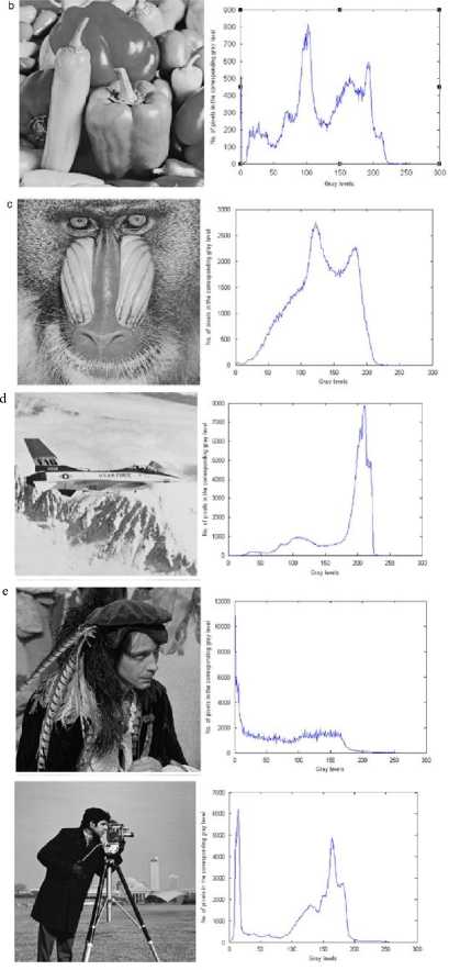
References A Fully Adaptive and Hybrid Method for Image Segmentation Using Multilevel Thresholding
- Sezgin, M., & Sankur, B.. ‘Survey over image thresholding techniques and quantitative performance’. Journal of Electronic Imaging, (2004) 13 146 – 165.
- Kittler, J., & Illingworth, J. Minimum error thresholding. Pattern Recognition, (1986) 19, 41–47.
- Wang, S., Chung, F. L., & Xiong, F. A novel image thresholding method based on Parzen window estimate. Pattern Recognition,. (2008) 41, 117–129
- Otsu, N. A threshold selection method from gray level histograms. IEEE Transactions on Systems, Man and Cybernetics SMC-9,. (1979) 62–66
- Kapur, J. N., Sahoo, P. K., & Wong, A. K. C. A new method for gray-level picture thresholding using the entropy of the histogram. Computer Vision Graphics Image Processing(1985),29, 273–28
- Yen, P-Y., A fast scheme for multilevel thresholding using genetic algorithms. Signal Processing. (1999) 72 85-95.
- Hammouche, K., Diaf, M., & Siarry, P., A multilevel automatic thresholding method based on a genetic algorithm for a fast image segmentation. Computer Vision Image Understanding. (2008) 109 (2) 163–175.
- Wu, B.-F., Chen, Y.-L., & Chiu, C.-C., Recursive algorithms for image segmentation based on a discriminant criterion, International. Journal. Signal Processing (2004) 1 55–60.
- Huang, D.-Y., & Wang, C.-H. Optimal multi-level thresholding using a two-stage Otsu optimization approach. Pattern Recognition Letters, (2009) 30 (3), 275-284.
- Wang, N., Li, X., & Chen, X. H. Fast three-dimensional Otsu thresholding with shuffled frog-leaping algorithm. Pattern Recognition Letters. (2010) 31 (13), 1809–1815
- Li, C. H., & Tam, P. K. S. An iterative algorithm for minimum cross entropy thresholding. Pattern Recognition Letters, (1998) 19 (8), 771-776
- Chung, K.-L., & Tsai, C.-L. Fast incremental algorithm for speeding up the computation of binarization. Applied Mathematics and Computation, (2009) 212 (2), 396-408.
- Yin, P. I Multilevel minimum cross entropy threshold selection based on particle swarm optimization’. Applied Mathematics and Computation. (2007) 184 (2), 503–513.
- Shelokar, P.S., Jayaraman, V.K, & Kulkarni, B.D. An Ant Colony approach for Clustering. Anal. Chim. Acta 59, (2004) pp 187–195
- Goldberg, D.E., Genetic Algorithms in Search, Optimization, and Machine Learning..Addison-Wesley, Reading, MA. (1989)
- Kennedy, J & Eberhart, R. C. Particle swarm optimization. In Proc.IEEE Int. Conf. Neural Netw, Perth, Australia,. (1995) 4, 1948–1972
- Storn, R., & Price, K. Differential Evolution — a simple and efficient heuristic for global optimization over continuous spaces. Technical Report TR-95-012.,ICSI. (1995)
- Kirkpatrick, S., Gelatt, C.D., & Vecchi, M.P. Optimization by simulated annealing. Science .220 4598, (1983) 71–680.
- Karaboga, D. An idea based on honey bee swarm for numerical optimization, Technical Report TR06, Erciyes University, Engineering Faculty, Computer Engineering Department. (2005)
- Passino, K.M., Biomimicry of bacterial foraging for distributed optimization and control. IEEE Transactions on Control Systems Magazine (2002) 22 (3), 52–67.
- Lai, C.-C., and Tseng, D.C A hybrid approach using Gaussian smoothing and genetic algorithm for multilevel thresholding. International Journal of Hybrid Intelligent Systems. ., (2004) 13, 143–152.
- Srinivas, M., & Patnaik, L.M. Adaptive probabilities of crossover and mutation in genetic algorithms, IEEE Transactions on Systems, Man and Cybernetics (1994) 24 (4).
- Cao,L.,Bao,P.,Shi,Z.,. The strongest schema learning GA and its application to multilevel thresholding Image and Vision Computing 146 (9–10), (2008) 387–390.
- Cuevas, E., Zaldivar, D. & Pérez-Cisneros, M. A novel multi-threshold segmentation approach based on differential evolution optimization. Expert Systems with Applications (2010) 37, 5265-5271.
- Rahnamayan, S., Tizhoosh, H.R., & Salama, M.M.A. Image thresholding using differential evolution. In: Proceedings of International Conference on Image Processing, Computer Vision and Pattern Recognition, Las Vegas, USA, (2006) 244–249.
- Sarkar, S, Gyana RanjanPatra, & Das, S. A Differential Evolution Based Approach for Multilevel Image Segmentation Using Minimum Cross Entropy Thresholding. SEMCCO (2011) 1. 51-58.
- Du, F., Shi, W. K., Chen, L. Z., Deng, Y., & Zhu, Z. Infrared image segmentation with 2-D maximum entropy method based on particle swarm optimization PSO’. Pattern Recognition Letters, (2005) 265, 597–603.
- Madhubanti, M., & Amitava, A. A hybrid cooperative-comprehensive learning based PSO algorithm for image segmentation using multilevel thresholding. Expert Systems with Application, (2008) 34, 1341–1350.
- Ye, Z. W., Chen, H. W., Li, W., & Zhang, J. P.. Automatic threshold selection based on particle swarm optimization algorithm. In Proceedings of international conference on intelligent computation technology and automation. 2008. 36– 39
- Zhang, R. & Liu, J. Underwater image segmentation with maximum entropy based on Particle Swarm Optimization PSO. In Proceedings of the first international multi symposiums on computer and computational Sciences IMSCCS’06, (2006). 360–363.
- Horng, M.-H. Multilevel thresholding selection based on the artificial bee colony algorithm for image segmentation. Expert Systems with Applications. (2011) 38, 13785-13791.
- Zhang, Y., & Wu, L. Optimal Multi-Level Thresholding Based on Maximum Tsallis Entropy via an Artificial Bee Colony Approach. Entropy, (2011) 134, 841-859
- Sathya, P. D., & Kayalvizhi, R. Modified bacterial foraging algorithm based multilevel thresholding for image segmentation. Engineering Applications of Artificial Intelligence, In Press SEAINPC. (2011) 65–69.
- Hammouche, K., Diaf, M., & Siarry, P. A comparative study of various metaheuristic techniques applied to multilevel thresholding problem. Engineering Applications of Artificial Intelligence, (2010) 23, 667–688.
- Bruzzese, D. & Giani, U. Automatic Multilevel Thresholding Based on a Fuzzy Entropy Measure. In Classification and Multivariate Analysis for Complex Data Structures, (2011) 125-133
- Yen, J.C., Chang, F.J. & Chang, S. A new criterion for automatic multilevel thresholding, IEEE Trans. Image 78.
- Sezgin, M., & Tasaltin, R., A new dichotomization technique to multilevel thresholding devoted to inspection applications, Pattern Recognition. Letters. (2000) 21 151–161.
- Djerou, L., Khelil, N., Dehimi, H. E., & Batouche, M. Automatic Multilevel Thresholding Using Binary Particle Swarm Optimization for Image Segmentation. 2009 International Conference of Soft Computing and Pattern Recognition, (2009). 66-71.
- S-Hosseini, H., Intelligent water drops algorithm for automatic multilevel thresholding of grey-level images using a modified Otsu’s criterion. Int. J. Modelling, Identification and Control, (2012) 15, 4, 241
- Al-Obeidat, F, Belacel,N, Carretero, J.A & Mahanti, P. An evolutionary framework using particle swarm optimization for classification method proaftn . Applied Soft Computing (2011) 11 (8) 4971–4980.
- Chen, S. & Luk, B.L. Digital IIR filter design using particle swarm optimisation, International Journal of Modelling, Identification and Control, (2010) 9 (4) 327–335.
- Poli, R, Analysis of the publications on the applications of particle swarm optimisation, Journal of Artificial Evolution
- Radha,T., Pant,M., Abraham, A., & Bouvry,P., Swarm Optimization: Hybridization Perspectives and Experimental Illustrations, Applied Maths and Computation, Elsevier Science, Netherlands, (2011) 217 (1) 5208-5226.
- Valdez, F, Melin,P, & Castillo, O. An improved evolutionary method with fuzzy logic for combining particle swarm optimization and genetic algorithms, Applied Soft Computing (2011) 11 (2) 2625–2632.
- Zhang, Y., & Wu, L. Optimal Multi-Level Thresholding Based on Maximum Tsallis Entropy via an Artificial Bee Colony Approach. Entropy, (2011) 134, 841-859
- Zhang, Y., Zhang, M. & Liang, Y.C.H. A hybrid Aco/Pso algorithm and its applications, International Journal of Modelling, Identification and Control,(2009) 8 (4) 309–316.
- Shi,Y., & Eberhart, R. C., A modified particle swarm optimizer. In Proceeding IEEE Congr. Evol. Comput., (1998) 69–73.
- Kennedy, J & Eberhart, R. C. A discrete binary version of the particle swarm algorithm, in Procs. of the Conf. on SMC97, Piscataway, NJ, USA, (1997) 4104-4109.
- Chaojun, D., & Qiu, Z., Particle swarm optimization algorithm based on the idea of simulated annealing, International Journal of Computer Science and Network Security, (2006) 6 (10) 152–157.
- Fang, L., Chen,P., & Liu, S. Particle swarm optimization with simulated annealing for tsp, in Proceedings of the 6th WSEAS International Conference on Artificial Intelligence, Knowledge Engineering and Data Bases (AIKED ’07), (2007) 206–210, World Scientific and Engineering Academy and Society (WSEAS), Stevens Point,Wis, USA,
- Wang, X., & Li,J Hybrid particle swarm optimization with simulated annealing, in Proceedings of the 3rd International Conference on Machine Learning and Cybernetics (ICMLC ’04), ., (2004) 4 2402–2405.
- Xia, W. J., & Wu, Z. M A hybrid particle swarm optimization approach for the job-shop scheduling problem, International Journal of Advanced Manufacturing Technology, (2006) 29 (3-4), 360–366.
- Yang, G., Chen, D., & Zhou, G., A new hybrid algorithm of particle swarm optimization, in Lecture Notes in Computer Science, (2006) 41 15, 50–60.
- Metropolis, N., Rosenbluth, A.W., Rosenbluth, M.N., &Teller, A.H. Equation of state calculations by fast computer machines, Journal of Chemical Physics (1953) 21 (6) 1087–1092.
