A fuzzy based parametric approach for software effort estimation

Author: H. Parthasarathi Patra, Kumar Rajnish
Journal: International Journal of Modern Education and Computer Science @ijmecs
Article in issue: 3 vol.10, 2018.
Free access
Accurate Software effort estimation is an ongoing challenge for the modern software engineers in computer science engineering since last 30 years due to the dynamic behavior of the software [1] [2][14]. This is only because of the time and cost estimation during the early stage of the software development is quite difficult and erroneous. So many algorithmic and non algorithmic techniques are used such as SLIM (Software life cycle management), Halstead Model, Bailey-Basil Model, COCOMO model and Function point analysis, etc, but does not estimate all kinds of software accurately. Nowadays these traditional techniques are not acceptable. This research work proposes a new fuzzy model to achieve higher accuracy by multiplying a fuzzy factor with the effort equation predicted empirically. As comparison to both model based and equation based, Model based estimation focused on specific models where as equation based techniques are based on traditional equations. Fuzzy logic is more suitable and flexible to meet the realistic challenges of today’s software estimation process.
Fuzzy logic, Membership function, KLOC, MRE, MMRE, PRED
Short address: https://sciup.org/15016746
IDR: 15016746 | DOI: 10.5815/ijmecs.2018.03.06
Text of the scientific article A fuzzy based parametric approach for software effort estimation
Published Online March 2018 in MECS DOI: 10.5815/ijmecs.2018.03.06
This paper focused to satisfy the need of today’s software industry by estimating the cost and effort and challenging the various issues and variations occurred in software size. Accuracy and timely estimation of software efforts is one of the most critical activities to manage a software project [7] [8]. As both over estimate and under estimate of software is very harmful for modern software industry this paper gives emphasis to predict the effort accurately and reliably. If the estimation is low then the software development team will be under pressure to finish the product and if the estimation is high then the most of the resources will be commuted to the projects [9][11][21]. It is very critical to implement novel methods to improve the accuracy of a software projects. So nowadays many models are used to estimate the efforts. This model proposed an extensive COCOMO [4] [5] [6] model by changing the scale factors and constant values a, b and multiplying a fuzzy factor to measure the software effort. This paper structured as follows: Section II describes the overview of existing techniques, Section III describes a frame work to estimate the efforts as comparing with COCOMO model, and Section IV relates the development tools and techniques and section V relates conclusion and future work.
-
II . Overview of Different Models Used for
Software Estimation
Since 1990 more than 20 different models are used to estimate the cost, effort, Duration and productivity of the software project [4] [5]. These are categorized as follows.
-
• Model based
-
• Expert Judgment
-
• Learning based
-
• Dynamic Based
-
• Regression Analysis
-
• Composite methods
-
A. Halstead Models
Halstead formulate a relation to estimate the effort as [3].
Effort ( E ) = 0.7 x ( KLOC ) 1.5 (1)
-
B. Bailey-Basil Model
Bailey and Basil formulate a relation to estimate the efforts [2].
Effort ( E ) = 5.5 x ( KLOC) 1.16 (2)
-
C. Walston -Felix Model
Walston and Felix developed a model to estimate the efforts taking 60 IBM projects and analyzing relationship between derived lines of codes, constitutes participation, customer oriented changes and new lines of code
Effort (E) = 5.2 x (KLOC) 0.91(3)
Duration (D) = 4.1 x (KLOC)0.36
-
D. Doty Model (Kloc>9)
Effort (E) = 5.288 x (KLOC )1.047
-
E. Sel Model
The software engineering laboratory (SEL) of the University of Maryland has established a model to estimate the effort as
Effort (E) = 1.4 x (KLOC )0'93
Duration (D) = 4.6 x (KLOC)0.26
-
F. Cocomo Ii Model
This model formulate like
Effort (E) = 2.9 x (KLOC )M(8)
-
III. Proposed Model and Methodology
Till now none of the existing models can measure software efforts accurately in the modern software industry for all kind of software’s. In this paper we analyze a new empirical model for effort estimation. The cost drivers which are very from project to project, so we have taken different scale factor values and categories the cost drivers into project, product, personal and computer. Finally by multiplying a fuzzy factor value the efforts are calculated.
-
A. Data Collection
For this paper the data’s are collected from 60 NASA projects from different containers, 93 NASA projects from common NASA2 and 63 NASA projects from promise repository. These data sets are real project data sets and may be used for practical proposes and can be viewed from “The Promise Repository of Empirical Software Engineering Data”. North Carolina State University, Department of Computer Science
-
B. Description About Proposed Model
This model is based on empirical analysis of 216 NASA Projects of different repository and it includes the scale factors like personnel, complexity, environment, risks and constraints. It predicts effort, cost estimates and reliability using the statistical approaches like y =a ×
(KLOC) + d to evaluate the cost, effort and duration empirically analyzing 216 real projects data of NASA. In this model we use a regression formula, with the parameters ‘a’ and ‘b’ which are derived from project dataset using deterministic and heuristic methods and optimizing the global solution. In this by the regression analysis we express the relationship between two variables and to estimate the dependent variable (i.e. Effort ) based on independent variable (i.e. LOC ) using simulated annealing algorithm [18].
Simulated annealing algorithm might have been used to solve a wide range of optimization problems in artificial intelligence and other areas. But in this study we have used it as a simple way to implement the algorithm to derive the parameters a, b considering randomly chosen values. However, it would be inappropriate to solve a complex problem to illustrate how to use simulated annealing [17]. Thus, we have taken a two variable function of Equation 9 and have been used for instructive purposes. There may have other optimization methods, which are more appropriate to solve this second order equation, but this section is only trying to set the basics for proper use of simulated annealing [10][18][19].
F ( x , У ) = x 2 + У 2 + 5 ХУ - 4 (9)
To get a better sense of the behavior of Equation 9, Fig. 1 shows the simulation graph of this equation. Let suppose that the goal is to find the values of x and y that minimize f(x, y). Clearly the solution is any point (x, y) that lies on the circle that intersects f(x, y) with the plane z = 0.We normally use simulated annealing when the solution has many variables, and finding or visualizing the solutions in these cases is much more difficult than interpreting the 3-D plot of Fig.1 [18][19][20]
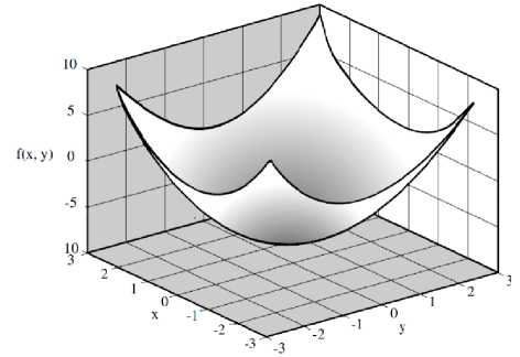
Fig.1. (Simulation Graph)
-
C. Proposed Algorithm Description
-
I. Start
-
II. Read the project KLOC and actual effort as E
-
III. Follow the equation E = n x a x ( KLOC)b where a, b are constants and n is the no. of projects.
-
IV. Z log( KLOC) + Z log E = n x A + B Z log ( KLOC)
-
V. Z log( KLOC ) xZ log( E ) = A xZ log( KLOC ) + B x ( Z (log( KLOC )))2
Where A=log (a) and B = b+1.
-
VI. Use the steps 4 and 5 to estimate the parameter Value of a and b by the method of statistical Techniques using the data of real projects empirically
-
VII. End.
-
D. Evolution Of Proposed Algorithm
Here the authors make a convenient way to estimate the effort and the new cost driver values are taken empirically as shown in Table 2 The proposed approach provides more accurate estimation with the comparison of COCOMO model. Researchers may redefine the value of cost drivers further for better result. Individually analyzing organic, semi detached and embedded projects empirically we got the parameter value a, b as shown in Table 1
Table 1. Predicted parameters for proposed model
|
Type |
A |
B |
a |
b |
|
Organic |
0.3560 |
2.03 |
2.27 |
1.03 |
|
Semi- Detached |
0.4623 |
2.14 |
2.9 |
1.14 |
|
Embedded |
0.4471 |
2.2 |
2.8 |
1.2 |
The formula used to calculate the effort is
Effort ( E ) = a x ( KLOC)b x П 1 = 1 NEAF x FF (10)
Where NEAF is the new effort adjustment factors, which are new cost driver calculated by the author in this paper empirically as shown in Table 2 and FF is the fuzzy factor will be calculated using Fuzzy Inference System as shown in Table 4.
-
E. Fuzzy Logic
Fuzzy Logic is based on four basic concepts Fuzzy sets, Linguistic Variables, Possibility distribution and fuzzy If-then rules. Fuzzy Sets are the sets with smooth boundaries like “Partha is Smart” [0, 1]. Linguistic variables – consider the sentence “Customer service is poor” uses a fuzzy set “poor” to describe the quality. Here Customer service is the linguistic variable. Possibility distribution means the constraints on the value of a linguistic variable imposed by assigning it a fuzzy set i.e. KLOC (Ranges) = [0, 300]. Fuzzy if-then rules are the conditional statement to describe a functional mapping that generalizes a bidirectional control structure in two-valued logic [22].
-
F. Fuzzy Inference Process
Fuzzification[12]: A membership function (MF) is a curve that defines how each point in the input space (universe of discourse) is mapped to a membership value (or degree of membership) between 0 and 1.
Logical Operators and if-then Rules : Fuzzy if-then rule statements are used to formulate the conditional statements for a specific output. For example a single fuzzy if-then rule assumes the form if x is M then y is N, Where M and N is linguistic values.
Defuzzification: There are two types of fuzzy inference systems in the fuzzy logic toolbox: Mamdani-type and Sugeno-type. In this model we have used Mamdani Type
Inference system
-
IV. Development Tools And Technique
In this paper we have used MATLAB 7.5 which is a high-performance language for technical computing. It integrates computation, visualization, and programming in an easy-to-use environment where problems and solutions are expressed in familiar mathematical notation. We have used the following properties of MATLAB in this paper.
-
> Math and computation
-
> Algorithm development
-
> Data acquisition
-
> Modeling and simulation.
-
> Data analysis, exploration, and visualization
-
> Scientific and engineering graphics using Fuzzy Logic
-
> Application development, including graphical user interface building.
-
> Fuzzy Interface System (Mamdani) in fuzzy logic Tool Box
-
A. Implementation
This research will implement the algorithm proposed by the author using the new effort drivers given in Table 2 using Mamdani Fuzzy Inference System (FIS) and the predicted effort will be compared with Constructive Cost Model (COCOMO). Fuzzy Triangular membership (trimf) function has been taken for implementation. The results were analyzed using the criterion MRE, MMRE (Mean Magnitude of Relative Error), RMSE and PRED.
-
B. Research Methodology Used
In this method we have selected a particular type of Fuzzy Inference System (Mamdani) as shown in Fig. 2 and define the input variables (KLOC and Mode) and output variable (Fuzzy Factor). Then we set the type of the membership functions for input variables and the type of the membership function for output variable as shown in Fig. 3, Fig. 4 and Fig. 5. Here we have used 37 rules in Rule Editor as shown in Fig.8 and the data is now translated into a set of if–then rules written in Rule editor. The detailed model structure is shown in the Fig. 6. The detail fuzzy frame work used is shown in Fig. 2.
Table 2. New Effort Adjustment Factor
|
Sl N o |
Cost Driver |
Very Low |
Low |
Nominal |
High |
Very High |
Extra High |
|
1 |
Required Reliability |
0.75 |
0.97 |
1 |
1.15 |
1.18 |
2 |
|
2 |
DB Size |
0.86 |
0.96 |
1 |
1.01 |
1.18 |
1.9 |
|
3 |
Product complexity |
0.7 |
0.99 |
1 |
1.19 |
1.2 |
1.23 |
|
4 |
Time constraint |
0.78 |
0.85 |
1 |
1.35 |
1.38 |
1.86 |
|
5 |
Main Memory constraint |
0.7 |
0.85 |
1 |
1.01 |
1.22 |
1.76 |
|
6 |
Machine volatility |
0.8 |
0.93 |
1 |
1.01 |
1.3 |
1.55 |
|
7 |
Turnaroun d Time |
0.8 |
0.93 |
1 |
1.09 |
1.34 |
- |
|
8 |
Analyst Capability |
1.46 |
1.19 |
1 |
0.86 |
0.78 |
- |
|
9 |
Applicatio n experience |
1.29 |
1.23 |
1 |
0.95 |
0.94 |
- |
|
10 |
Programm er capability |
1.42 |
1.17 |
1 |
0.96 |
0.95 |
- |
|
11 |
Virtual Machine |
1.34 |
1.01 |
1 |
0.82 |
- |
- |
|
12 |
Language experience |
1.02 |
0.98 |
1 |
0.92 |
- |
- |
|
13 |
Modern programmi ng practice |
1.24 |
1.14 |
1 |
0.94 |
0.81 |
- |
|
14 |
Use of software tools |
1.19 |
1.14 |
1 |
0.93 |
0.82 |
- |
|
15 |
Schedule constraint |
1.23 |
1.03 |
1 |
1.08 |
1.1 |
- |
Mode
Fuzzy Factor
Size (KLOC)
Rules
Fig.2. Frame work for Fuzzy Interface System
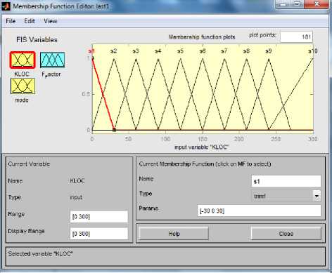
Fig.3. MF for input variable KLOC
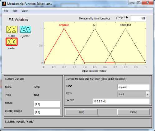
Fig.4. MF for input variable Mode
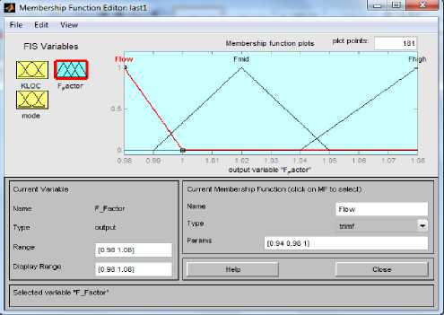
Fig.5. MF for output variable Fuzzy Factor
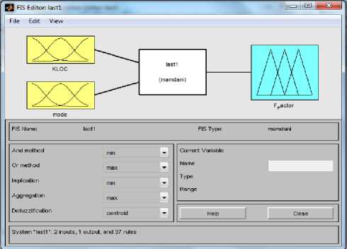
Fig.6. Fuzzy Inference System
-
C. Performance Of The Proposed Model
Table 5 shows the result of effort estimation by the proposed model as comparison to COCOMO model and Table 3 shows the effort variance of different model in accordance with the data of 15 given projects and measure the performance to validate the outcome. Table 4 shows the performance of the proposed model using MMRE, RMSE and PRED with comparison to COCOMO models.
Table 3. Effort Variance of different Models
|
KLOC |
Actual Effort |
COCOMO Basic % |
COCOMO Inter % |
Proposed % |
|
25.9 |
117.6 |
14.23 |
14.23 |
3.91 |
|
24.6 |
117.6 |
19.03 |
19.03 |
1.95 |
|
7.7 |
31.2 |
16.9 |
16.9 |
2.8 |
|
8.2 |
36 |
2.27 |
2.27 |
8.3 |
|
2.2 |
8.4 |
24.16 |
24.16 |
6 |
|
66.6 |
352.8 |
17.65 |
17.65 |
0.73 |
|
11.3 |
36 |
22.5 |
22.5 |
1 |
|
15 |
48 |
38.5 |
38.5 |
5.6 |
|
15 |
90 |
30.8 |
30.8 |
0.55 |
|
16.3 |
82 |
19.19 |
19.19 |
3.6 |
|
14 |
60 |
15.76 |
15.76 |
1 |
|
16 |
114 |
25.04 |
25.04 |
3.5 |
|
50 |
1024 |
74 |
5.1 |
8 |
|
90 |
162 |
128.7 |
7.7 |
2.9 |
|
41 |
599 |
40.23 |
53.51 |
1 |
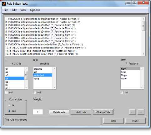
Fig.8. Rule Editor of Fuzzy Interface System
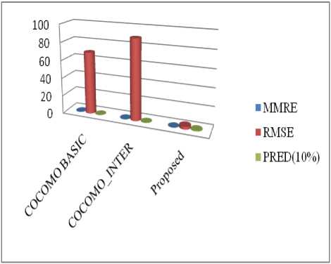
Fig.7. Performance Graph (COCOMO Vs Proposed Model
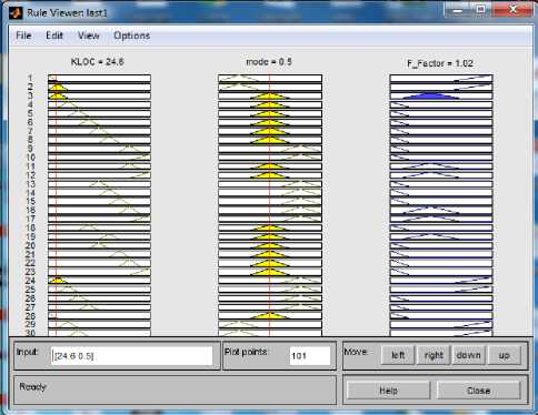
Fig.9. Rule viewer of FIS
Table 4 Performance of COCOMO VS Proposed Model
|
Performance |
COCOMO Basic |
COCOMO Inter |
Proposed Model |
|
MMRE |
0.2436 |
0.25185 |
0.03512 |
|
RMSE |
69.07 |
89.22 |
3.11 |
|
PRED (10%) |
0.16 |
0.25 |
1 |
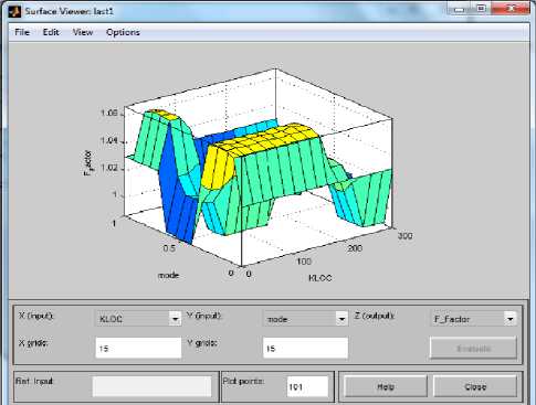
Fig.10. Surface viewer of Fuzzy Factor
-
D. Evaluation Criteria And Error Analysis [16].
There are so many statistical approaches are used to estimate the accuracy of the software effort. We are using methods like MRE, MMRE, RMSE, and Prediction. Boehm [2] suggested a formula to find out the error percentage as shown below
Pr edicted Effort - Actual Effort
Error % = _ _^-- (11)
Actual _ Effort
MRE (Magnitude of relative error): We can calculate the degree of estimation error for individual project.
| Pr edicte Effort - Actual Effort |
MRE =J----------------------1 (12)
Actual _ Effort
RMSE (Root Mean Square Error): we can calculate it as the square root of the mean square error and can be defined as.
RMSE = .-£n i( Actual Effort - Pr edicted Effort )2 (13) V n i = 1
MMRE (Mean Magnitude of Relative Error): It is another way to measure the performance and it calculates the percentage of absolute values of relative errors. It is defined as.
MMRE = 1 Yn | Pr edicted _ effort - Actua1 _ Effort | n i = 1 Actual _ Effort
PRED (N): This criteria is used to calculate the average percentage of estimates that were within N% of the actual values i.e. the percentage of predictions that fall within p % of the actual, denoted as PRED (p).Where k is the number of projects in which MRE is less than or equal to p, and n is the total number of projects. It is defined as PRED (p) = k / n
For project1 having KLOC =25.9 the actual effort is 117.6 Man-Month and the calculated effort for Basic COCOMO and Intermediate COCOMO is 100.86 MM and by the proposed model is 122.2 MM. Similarly for project 2 KLOC=24.6 the actual effort is 117.6 MM and calculated effort for Basic COCOMO and Intermediate COCOMO is 95.21 MM and by the proposed model is 115.3 MM. Now we can calculate the % of error using the equation 11. For project 1, the error % for Basic COCOMO and Intermediate COCOMO is (-14.23) % and error % for proposed model is (+3.91) %. Similarly For project 2, the error % for Basic COCOMO and Intermediate COCOMO is (-19.03) % and error % for proposed model is (-1.95) %. Here the negative % indicates the under estimation of the project and positive % error indicates the project is over estimate. Big under estimate gives extra pressure to the developing staff and leads to add more staffs which causes the late to finish the project. According to Parkinson’s Law “Work expands to fill the time available for its completion” Big over estimation reduces the productivity of personnel’s [15]. So during estimation the researchers should have to give emphasis to reduce the big over or under estimation of the project.
-
E. Comparison With Cocomo Models[13]
In software estimation COCOMO model is a regular and standard model to estimate the effort developed by Barry Boehm. But in the proposed model the researcher used a basic regression formula, with parameters that are derived from historical project (NASA software). Here we are estimating the effort based on the actual project characteristic data and better result predicts as compare to MMRE and RMSE as shown in Table 4.
-
F. Advantages Of Proposed Model
-
> It Is reusable
-
> It calculates software development effort as a function of program size expressed in Kilo Lines of code (KLOC)
It predicts the estimated effort with more accuracy.
-
V. Conclusion And Future Work
This proposed model can be useful to estimate the software effort with better accuracy which is very important when software pays a lot in every industry. In this paper the author analyze more than 250 projects collected from PROMISE repository. The predicted result shows there is very close values between actual and estimated effort. The effort variance is very less and the proposed model has the lowest MMRE and RMSE and prediction values i.e. 0.03512 and 3.11 and 1.0 respectively. So the proposed model may able to provide good estimation capabilities for today’s software industry. A fuzzy model is more adaptive when the systems are not suitable for analysis by conventional approach or when the available data is uncertain, inaccurate or vague. The major difference between our work and previous works is that two fuzzy logic functions will be used for software development effort estimation on the model and then it’s validated with gathered data. The advantages of fuzzy logic are combined and learning ability and good generalization are obtained. The main benefit of this approach is it has good interpretability by using the fuzzy rules. The effort predicted using four fuzzy logic functions will be compared with Intermediate COCOMO.
Table 5. Effort estimation by different Models
|
Sl. No |
Mode |
KLOC |
Actual Effort |
Fuzzy Factor |
Proposed Effort |
COCOMO Basic |
COCOMO Inter |
|
1 |
SD |
25.9 |
117.6 |
1.02 |
122.2 |
100.86 |
100.86 |
|
2 |
SD |
24.6 |
117.6 |
1.02 |
115.3 |
95.21 |
95.21 |
|
3 |
SD |
7.7 |
31.2 |
1.01 |
30.3 |
25.92 |
25.92 |
|
4 |
SD |
8.2 |
36 |
1.01 |
33 |
27.81 |
27.81 |
|
5 |
SD |
9.7 |
25.2 |
1.01 |
39.3 |
33.57 |
33.57 |
|
6 |
SD |
2.2 |
8.4 |
0.999 |
7.89 |
6.37 |
6.37 |
|
7 |
SD |
3.5 |
10.8 |
1 |
12 |
10.72 |
10.72 |
|
8 |
SD |
66.6 |
352.8 |
0.997 |
350.2 |
290.5 |
290.5 |
|
9 |
SD |
7.5 |
72 |
1.02 |
66.38 |
40.9 |
40.9 |
|
10 |
SD |
20 |
72 |
1.02 |
62.8 |
32.98 |
32.98 |
|
11 |
SD |
6 |
24 |
1 |
15.7 |
10.52 |
10.52 |
|
12 |
SD |
100 |
360 |
0.987 |
378 |
200 |
200 |
|
13 |
SD |
11.3 |
36 |
1.01 |
36.37 |
27.9 |
27.9 |
|
14 |
SD |
20 |
48 |
1.02 |
63.47 |
68.76 |
68.76 |
|
15 |
SD |
15 |
48 |
1.01 |
45.27 |
29.35 |
29.35 |
|
16 |
SD |
19.7 |
60 |
1.01 |
88.3 |
72.24 |
72.24 |
|
17 |
SD |
66.6 |
300 |
0.987 |
343.9 |
264.54 |
264.54 |
|
18 |
SD |
29.5 |
120 |
1.02 |
141 |
116.6 |
116.6 |
|
19 |
SD |
15 |
90 |
1.01 |
90.5 |
62.21 |
62.21 |
|
20 |
SD |
38 |
210 |
1.02 |
229.5 |
182.5 |
182.5 |
|
21 |
SD |
10 |
48 |
1.01 |
33 |
30.95 |
30.95 |
|
22 |
SD |
15.4 |
70 |
1.01 |
73.3 |
62.17 |
62.17 |
|
23 |
SD |
48.5 |
239 |
1.01 |
273.9 |
224.7 |
224.7 |
|
24 |
SD |
16.3 |
82 |
1.01 |
79 |
66.26 |
66.26 |
|
25 |
SD |
12.8 |
62 |
1.01 |
59.9 |
50.54 |
50.54 |
|
26 |
SD |
32.6 |
170 |
1.02 |
175 |
144.02 |
144.02 |
|
27 |
SD |
35.5 |
192 |
1.02 |
193.8 |
158.44 |
158.44 |
|
28 |
SD |
5.5 |
18 |
1 |
20.65 |
17.78 |
17.78 |
|
29 |
SD |
10.4 |
50 |
1.01 |
43 |
36.3 |
36.3 |
|
30 |
SD |
14 |
60 |
1.01 |
60.6 |
50.64 |
50.64 |
|
31 |
SD |
6.5 |
42 |
1.01 |
34 |
32.28 |
32.28 |
|
32 |
SD |
13 |
60 |
1.01 |
64.6 |
61.01 |
61.01 |
|
33 |
SD |
90 |
444 |
0.986 |
448.6 |
360 |
360 |
|
34 |
SD |
8 |
42 |
1.01 |
37.3 |
35.42 |
35.42 |
|
35 |
SD |
16 |
114 |
1.01 |
110 |
85.45 |
85.45 |
|
36 |
SD |
177.9 |
1248 |
1355 |
1.01 |
1152 |
1152 |
|
37 |
E |
70 |
458 |
1.05 |
454 |
606.44 |
471.6 |
|
38 |
E |
271 |
2460 |
1.01 |
2222 |
1994 |
2393.9 |
|
39 |
E |
60 |
409 |
0.986 |
470 |
497.9 |
387 |
|
40 |
E |
100 |
703 |
0.987 |
832 |
602 |
714.9 |
|
41 |
E |
32 |
1350 |
1.07 |
1201 |
1557.5 |
1211 |
|
42 |
E |
53 |
480 |
1.07 |
656 |
281.4 |
612 |
|
43 |
E |
41 |
599 |
1.01 |
605 |
358 |
278.47 |
|
44 |
E |
24 |
430 |
1.07 |
337 |
188.29 |
146.45 |
|
45 |
E |
165 |
4178 |
1.05 |
3787 |
1099 |
3555 |
|
46 |
E |
65 |
1772 |
1.06 |
1250 |
359.5 |
1162.6 |
|
47 |
E |
70 |
1645 |
1.05 |
1255 |
392.9 |
1105 |
|
48 |
E |
50 |
1024 |
1.07 |
942 |
262.4 |
1077 |
|
49 |
Organic |
90 |
162 |
1.07 |
157.2 |
370.6 |
174.54 |
|
50 |
Organic |
240 |
192 |
0.986 |
371 |
1111.8 |
522 |
References A fuzzy based parametric approach for software effort estimation
- Zia, Z.; Rashid, A “Software Cost Estimation for component based fourth-generation- Language software applications”, IET software, vol.5 (2011), pp. 103-110
- Boehm, B. W. and Papaccio, P. N “Understanding and controlling software costs,” IEEE Transactions on Software Engineering, vol. 14(1988), no. 10.
- Benediktsson, O. and Dalcher, D. “Effort Estimation in incremental Software Development,” IEEE Proc. Software, Vol. 150, no. 6(2003), pp. 351-357.
- Boehm, B.W. “Software engineering economics” (1981), Prentice –hall.
- Srivastava, D.K.; Chauhan, D.S. and Singh,” R,Square Model- A Software Process Model for IVR Software System”- International Journal of Computer Application (0975-8887) Volume 13- No 7.(2011), 33- 36.
- Jørgensen, M. and Sjøberg, D.I.K. “The impact of customer expectation on software development effort estimates,” International Journal of Project Management, 22(4) (2004): pp. 317-325.
- Seth, K and Sharma, A. “Effort Estimation Techniques in Component based Development”- A Critical Review Proceedings of the 3rd National Conference, (2009) INDIACom.
- Shepperd, M. and Schofield, C. “Estimating Software Project Effort Using Analogies,” IEEE Transactions on Software Engineering, vol. 23, no. 12(1987), pp. 736-743..
- Maxwell, K.D. and Forselius, P.”Benchmarking Software Development Productivity” IEEE Software, 17 (2000): pp. 80- 88.
- Uysal, M. “Estimation of the Effort Component of the Software Projects Using Simulated Annealing Algorithm,” World Academy of Science, Engineering and Technology. (2008)
- Moløkken-Østvold, K. and Jørgensen, M. “A Review of Surveys on Software Effort Estimation.” ACM-IEEE International Symposium on Empirical Software Engineering. Frascati, Monte Porzio Catone (RM), ITALY: IEEE. (2003) pp. 220- 230
- Attarzadeh,“A Novel Soft Computing Model to Increase the Accuracy of Software Development Cost Estimation,” The 2nd International Conference on Computer and Automation Engineering ICCAE, (2010) p. 603-607
- Singh, Y. and Aggarwal, K.K. “Software Engineering” Third edition, New Age International Publisher Limited New Delhi.(2005)
- Deshpande, M.V. and Bhirud, S.G. “Analysis of Combining Software Estimation Techniques,” International journal of Computer Applications (0975 – 8887) Volume 5 – No.3.
- Jolte, P. “An Integrated Approach to Software Engineering.” Third edition Narosa Publishing house New Delhi.
- Pressman. “Software Engineering - a Practitioner’s Approach”. 6th Edition McGraw Hill international Edition, Pearson education, ISBN 007 -124083.
- Suri, P.K.; Bharat, B. Time Estimation for Project Management Life Cycle: A Simulation approach, International Journal of Computer Science and Network Security, VOL.9 No.5. (2009)”
- Sergio, L.; Gabriel, A. and Raul, S.”Practical consideration of simulated annealing Implementation”, Cher Ming Tan (Ed.), ISBN: 978-953-7619-07-7 (2008).
- Montaz, A.; Aimo, T. and Sami, V”A Direct search simulated annealing algorithm for optimization involving continuous variables ”Turku center of computer science, Technical Report No-97(1997).
- Tushar, G. and Nielen, S.”Adaptive simulated annealing for global optimization”, Livermore software technology corporation, USA, 7th European LS-DYNA conference ,(2009).
- Ziauddin, Shahid K., Shafiullah K. and Jamal A. N. (2013) “A Fuzzy Logic Based Software Cost Estimation Model “International Journal of Software Engineering and Its Applications Vol. 7, No. 2.
- Babuska, R. “Fuzzy Modeling and Identification Toolbox User’s Guide” (August 1998).
