A game based energy sensitive spectrum auction model and bid learning process for cognitive radio systems

The huge shift to wireless communications brought about by the advent of smartphones and related devices is leading to congestion of the radio spectrum. The cause of the congestion is however mainly associated with the traditional fixed spectrum allocation schemes put in place by the different regulatory authorities [1, 2]. This led to the concept of Dynamic Spectrum Access (DSA) as proposed in [3]. Furthermore energy efficiency is a key factor in future wireless network because of climate change [4, 5]. In addition to this, the concept of Cognitive Radio Networks (CRN) has also been proposed in [6]. Consequently to complement the dynamic network, increase the revenue in relation to the increase in demand for expansion purposes and management of the occasional congestion as a result of people congregating in a single location such as during a football match, the Olympics or other events, dynamic pricing using the concept of an auction was also introduced. An auction process is important because, over the years the price paid for the spectrum has been based on potential price rather than allowing competition to reflect the actual price for the radio spectrum. Hence, this resulted into a growth in demand for the radio spectrum without a corresponding growth in revenue [7].

The implementation of a heterogeneous network requires proper planning in terms of pricing, licensing period and the power allocation mechanism among others to deliver the expected gain. However, the primary users of the radio spectrum are still not willing to share the radio spectrum based on the concept of DSA. This is because of concerns about interference from secondary users. Therefore, to encourage the efficient use of the radio spectrum for secondary access, [8] has previously – 695 – proposed the use of the green payments (GP) as an incentive for efficient use of the radio spectrum in and an auction based balancing on revenue and fairness was proposed in [9]. This paper uses the already proposed green paymnets to fomulate this work. This paper also examines a novel concept of a game based model in combination with an auction process to characterise the interactions that exist between the different competing elements in an auction based DSA network. This is done to reduce the amount of energy consumed in the system. The use of these two concepts to model a DSA network can also be found in [10-13].

The remaining parts of this paper are organised as follows: Section II defines some of the new and important models used in this paper. Section III defines the utility function adopted. Section IV shows a modelling scenario with the game model. Section V gives the results and discussion while the last section is the conclusions and future work.

• II.    System Model and Parameters

To model a heterogeneous network, the users in this paper are divided into two groups, the High Powered Users (HPUs) and the Low Powered Users (LPUs). The HPU requires a higher quality of service when compared to the LPU. Just these two categories are compared for simplification purposes. Furthermore we consider the presence of the service provider called the Wireless Service Provider (WSP) whose responsibility is to provide radio spectrum access to the users. These three entities considered form the players in the game model.

The Energy Model

The energy model is represented as a 2 state Markov chain shown in Fig. 1 and explained thus:

• 1.    A user who has file(s) to send moves into the OFF state and continue to be in this state until such user is among the winning bidders.

• 2.    A user who is among the winning bidders moves from the OFF state to the ON state.

• 3.    The user remains in the ON state until after transmission if transmission is successful or until when the user receives a failed signal either due to low offered bid compared to the reserve price or due to poor quality channel.

• 4.    After transmission the user moves back to the OFF state before switching completely off if no file is to be sent again. However if the user has another file to send, the user remains and attempt again in the off state. The complete off mode (not in Fig. 1) is the mode a user is in when there is no file to be sent.

A processing time which is the time taken to process the received bid is also assumed. All users that move from the ON state to the OFF state have the same processing time.

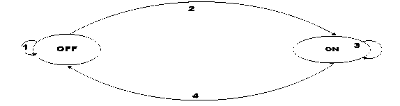
Fig. 1. Energy and system model as a two state Markov chain

The Reserve Price

The reserve price is the minimum price to be paid by any user intending to transmit before the spectrum is allocated to such a user. When the demand is low the reserve price helps to retain the minimum selling price of the WSP as shown in [8]. It is formulated by taking into account the current traffic load in the system, the frequency band, the total number of channels and the number of channels in use as:

RP(PriceUnit) = CfNTCCr.

Where C_r is a constant in price unit which is used to specify the value of a spectrum band in use. This value is determined from the common knowledge regarding the common price of the radio spectrum and it is specified in parameters Table 1. The users believe that the bigger the size of the network, the better the quality of service offered hence, the total number of channels in the system is also taken into consideration when calculating the reserve price. The congestion factor ( C f ) as shown below is introduced because of the laws of demand and supply as explained in [14]:

p _ ^N USA ^    N ac

.

The Users Bid

In an auction process, the bid of a user is important as it determines if the user wins or loses at the end of the process. To simplify the bid generation process, a concept called the Offered Bid Bin (OBB) is introduced. The OBB is like a lottery/raffle basket containing different bid values. A bidder dips into the bin (depending on the belief of the user) and picks a bid value. It is assumed that A_bs bins are available in the system and they are arranged in an ascending order. Each bin contains a specified range of continuous values (OBB₁ <  OB B₂< OBB₃ ... OBB_Abs . This means that a bid picked from OBB₂ is greater than a bid from a bid picked from OBB^ (bf^BB1< b°^BBz< Ь°^ВВз b_t^Abs ). Where b_t^Abs is the bid value picked by user i from OBB_Abs .

A user intending to seek access to the radio spectrum picks a bid from any of the bins depending on the user’s belief regarding the values of the bids submitted by other users in the system. It is quite similar to the traffic load bin used in [15]. However, unlike in [15] where the bids are assumed to be a discreet value, here the values are real numbers. The OBB is formulated as explained because the assumption in [15] that a user knows the system’s traffic load might not always be true, as such information is available mainly to the WSP.

The Users Belief

As stated earlier, the offered bid of a user depends on the belief of the user regarding the bids of others. Two beliefs models are proposed, the greedy and the learning model.

The Greedy or Non-learning Process

A user using the greedy model is assumed to be myopic and only intends to maximise its utility by bidding using a low price value. Such a user is known as extremely price sensitive bidder [16]. The bidder does not mind wasting energy by losing the auction process. Hence, it is assumed here that such a user is not learning the bid of the others or the reserve price.

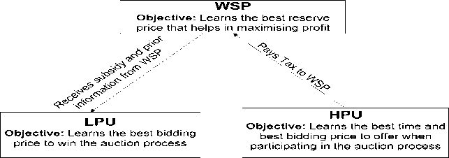
Fig. 2. Summary of the learning process

The Learning Process

Learning about the optimal bidding price can be useful to control the traffic load in the system especially when the system is congested in addition to the reduction in consumed energy and delay as demonstrated in [17]. Users that use the learning model are assumed to be interested in always winning or not wasting energy.

LPU Learning

A LPU receives a form of subsidy using the green payment equation as explained in [8] (while the HPUs are taxed using the same green payment equation). It is assumed that the LPU are provided with the information about the previous bids of the HPU in additional to the incentive received from the WSP. This information is used by the LPU as the prior information during the learning process. The WSP provides such information only to the LPU because as shown in [8] the WSP prefers the LPU transmitting rather than the HPU to keep interference in the system low.

HPU Learning

A HPU can only learn about the bids of the LPU based on an estimated prior knowledge while using the Bayesian learning model [18]. The HPU learn to understand when the LPU are not transmitting to increase their chances of winning the auction process (Fig. 2).

WSP Learning

The information available to the WSP is the bids submitted by the users. The aim of the WSP is to maximise revenue. Therefore, the WSP learns the user’s reservation price. The reservation price is determined by the user’s budget as explained in [19]. If the reserve price is higher than the user’s reservation price then no user is able to pay hence, the spectrum is not utilised. On the other hand, if there is congestion in the system, the WSP can increase the reserve price to prevent more users attempting to transmit.

• III.    The Utility Function

The utility function plays an important role in determining the achievable performance of a system. It describes the level of satisfaction or the preference of a user based on the QoS received [20]. It can be used in radio resource management to determine the level of satisfaction of the – 698 – users. The utility function can be described using different ways, but the choice of the function ........T is critical in achieving the desired performance. In this paper, it is defined for each set of" players using a power utility function because of its rapidly increasing nature. All the players are assumed

.......                        „.

to be rational and they seek to maximize their utility. The utility function of the users is divided into four parts: the utility based on the bid value ( U_B ), the utility based on the OBB ( U_OBB ), the utility based on the energy consumed per file sent ( U E ) and the utility based on the green payments ( U r)

Utility in Terms of the OBB

The higher the OBB a user picks a bid from, the lower the utility of the user in terms of the OBB. This means that a user that picks a bid from OBB 1 has a higher utility value in terms of the OBB compared to a user that picks a bid from OBB 2 or higher (U[OBB_A ) <  U(OBB_{A t}) .„., U(OBB₂) <  U(OBB₁)).

DS

This is because it is assumed that the users are price sensitive and the users aim is to win with the least possible amount. ___

U„„ = 2^^-l.                                (3)

Where OBB i is the bin where user i picks a bid and kgg_Abs is the bin containing the maximum possible bids. The bin (kgg_Abs ) that contains the set of maximum possible bid values has the least utility. OBB_Abs+1 ^is used ^{as the} denominator in order ^to avoid a user picking a ^bid from ^OBBA and huvinga utility of zero.

Utility in Terms of the Actual Offered Bid

The utility in terms of the actual offered Oid allows us to differentiate between users picking a low value of the bid to those picking a high value from the same OBB. As an illustration, a user offering a bid of 5.55 picked from OBB 5 has a lower utility compared to a user picking 5.95 from the same bin. The utility is formulated as shown below, where set NWU represents the winning bids in a bidding round

Nwu = ^bl,b2,b3^bNw^,

| (max(N wu ) - min(N wu ) for b_t<  max (Nwu) Omax N wu + d_k- min (Nwu) f or b = max (Nwuf

{ Max(N _wu )-bi

²     * 0    ^-1

Ifabidderwms otherwise

bi is the bid of any user i . If a bidder is not among the winning bidders, the utility of such a user is zero. The lower part of equation 5 contains a fixed value d_k which is specified in the parameter table. This is used for the user with the maximum bid to prevent a user from having a utility funct i on value of zero. The value of d_k is picked to be quite small so that it does not affect the utility of the highest bidder.

Utility in 'Terms of Energy Consumed During the Bidding Process

.                              • •                            .....            •

From the energy model, the more efficient a user is in terms of offering a bid that is accepted by the WSP, the more energy efficient the user is. A user whose bid is never rejected is considered to be more energy efficient compared to a user whose bid is sometimes/often rejected. This is because a user can only participate in the bidding process when in the ON state as explained earlier. It is measured as shown below:

^ES] U _e = 2Vnfg ) - 1.

Where N FS is the number of times a user has sent a file successfully, N FG is the number of times a user i has attempted to send a file but the users bid was rejected as a result of price. A rejected bid as a result of other factors (apart from price) is not considered as part of F i .

Utility in Terms of the Green Payments

The concept of the green payments was formulated in [8]. The utility in terms of the green payments is set to determine the satisfaction of the user depending on the value of the received green subsidy. The higher the amount of green payments subsidy received, the higher the utility of a user in terms of the green payment. However, it is assumed that a user paying a tax has a utility value of zero in terms of the green payment. This is done to allow for the simplification of this work rather than having a negative utility.

U J^x - I for Green Subsidy R l о      ForGreentax ,

R i is the green payment tax/subsidy for user i respectively, R max is the maximum subsidy.

The Overall Utility of the User

The overall utility of each of the user can vary between 0 and 1as shown below:

U =

^Ur+Uqbb _+Ub+Ue

2+-      .

ш

Where ω can vary between 1 and 2. This is done in order to vary the impact of U_R and U_OBB on the utility value. ω is specified in the parameters Table 1. It is introduced to reduce the weight associated to the utility in terms of the green payments and the OBB because it is assumed that they have less impact on the general utility of the users in this model. The components of the utility function that has less impact depend on the on the service offered by the system. This is because the satisfactions derived by users vary with the offered service. The peak point in Fig. 3 might be difficult to achieve because a user might prefer one factor more than the others, depending on the application in use. It can be as shown below.

Utility of the WSP

The utility of the WSP is based on the total revenue obtained. It is as shown below:

«GAU®

Ui(t)=2 NTC(t) -1.

Where N CAU ( t ) is the total number of channels that was available and used up till time t and N TC ( t ) is the total number of channels that was available in the system up till time t . It is assumed that if a channel is not occupied, the WSP is losing some revenue.

Table 1. Parameters used

Parameters	Value
Cell radius	2 km
Interference threshold	-40 dBm
Users in a cell	200
Number of cell	19
Noise floor	-114 dB/MHz
SINR max	21 dB
SINR threshold	1.8 dB
Cr	0.7
Max number of channels per cell	4
Height of base station	15 m
Height of mobile station	1 m
Budget	100000 Price Units
Transmit power for users	0.9 W/bit
Energy consumed by device	0.5 Watt sec
Power used in bidding	0.25% of the transmit power
A bs	12
d k	0.001
ω	1

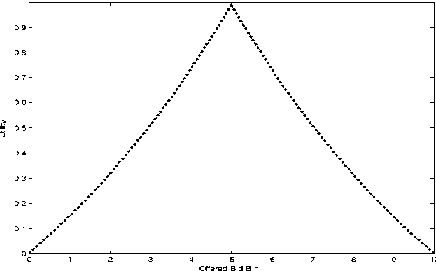
Fig. 3. Illustration of the Utility Function

• IV.    The Modelling Scenario

A cognitive network with users seeking access to the spectrum in an opportunistic manner is modelled, where N USA out of the possible N users in the system are competing for N AC unlicensed channels (where N_AC is the number of available channels). A multi-channel scenario ( N_AC > 1) is modelled using an uplink scenario. The bid of each user is either taxed or subsidized using the concept – 701 –

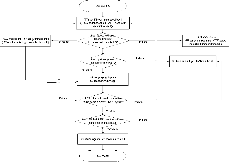
Fig. 4. System Flow Chart of green payments as described in [8]. The channel is allocated to the highest bidder(s) represented as NWU using the first price sealed bid auction with a reserve price as explained in [21]. The WINNER II B2 propagation model is used as detailed in [22]. The parameters used in the simulations are as given in Table 1.

The truncated Shannon equation is used to model the transmission rates of each of the users as detailed in [23]. The flow chart is as shown below (Fig. 4).

The Game Model

The game model is used to examine the utility of the learning users compared to the non-learning users. This section also investigates if a player can increase their utility by unilaterally changing from the learning model to the non-learning model or the other way round. The already formulated utility functions as explained are used.

A game model is used to study the allocation of the spectrum to obtain a satisfactory and a fair energy efficient auction based mechanism. This paper assumes a game which can be represented as a tuple G = [P, A, U]. Where P represents the set of players in the game, A represents the set of actions that is available to the players and U is the payoff or the utility obtained by taking an action. The players are represented as P = [GHPU, GLPU, W]. Where, GHPUrepresents the HPU, GLPUrepresents the LPU and W represents the WSP. Two actions are available to the players to either learn or use the greedy/non-learning approach A = [Al, Ag]). Each of the players aim is to maximise the obtained utility by bidding using the bid value that offers the maximum possible utility. The utility of the WSP depends on the revenue received as explained earlier. The players in the same group form a coalition using transfer learning. In this coalition, they share information such as the optimal OBB with each other. The aim of the game is to examine how a Nash Equilibrium can be achieved.

Each group of players can choose different actions ( A^l or A^g ) but the players in the same group can only choose or use the same action in an auction round. This means that if the G LPU decides to learn, all the users in the group are learning. If G_LPU is not learning then no user in that group can decide to learn. This is the same for G HPU and the WSP.

In the game formulation, a player belonging to G_LPU learns the optimal bid value by learning based on the prior probability provided by the WSP using Bayesian learning or adopting the greedy model. Each G_HPU can decide not to use the greedy model by learning the likelihood of being among the highest bidder and stays out if the likelihood is low. Depending on the value of the likelihood, the number of HPU that should attempt to bid during the next bidding round is determined. The equation of the likelihood is formulated such that the number of HPU attempting depends on the available channels and the offered bid of the users. This prevents a situation where the users are attempting to access the channels with either a low value of offered bid or when few channels are available in the system. This is because in such scenarios, it is most likely that the channels would be allocated to the LPU who are also attempting during the same bidding round. The formulation is as shown below:

Pr(i) = ( bi"bm )Nusa-NacNssa > Nac .                                   (11)

V max -b m

Where b m is the value of the reserve price if known to the user otherwise it is the minimum possible bid by user i based on the budget of the user. V max is the maximum possible valuation for a user per file and b i is the bid for user i . The probability is calculated for all the HPU users. If the probability is high for all the HPU attempting to transmit, then they are allowed, but if it is low, only a fraction are allowed as shown in equation (12). The users allowed are picked in descending order of the probability. The numbers allowed depend on the arriving users and the numbers of channels available. This is because at low traffic loads more HPU can be allowed, the numbers allowed decrease as the traffic load increase. It is as shown below:

N Usahpu^ WSahpuW .                             (12)

Where NUySAHPU(t) is the total number of HPU who arrived and wants to transmit during a transmission period t, NUSAhpu is the number of arriving HPU that are allowed to attempt to transmit after multiplying by the probability and Pr here is probability calculated from equation (12). This shows that the higher the likelihood, the higher the number of HPU allowed into the system. However, using the equation to determine the number of users allowed is not optimal. Therefore, the HPU varies the probability (Pr) in equation 12 and learns the optimal value for each traffic load provided Pr is positive initially. The equation is used in generating the prior probability and it serves as basis for the learning process. The HPU users use Bayesian learning as explained in [17] to learn the optimal number of users to be admitted into the system by exploring different numbers starting from the minimum provided by equation 12. Furthermore, the WSP also learns the traffic load which is used to fix the reserve price. When the system is congested (at traffic load of 4 Erlangs and above) the reserve price is fixed in such a manner that only bids from the highest OBB can be above the – 703 – reserve price. Therefore, the HPU paying the green tax are denied complete access to the spectrum. In this model it is assumed that that WSP is also learning the traffic load in this system using that Bayesian learning model in order to fix the appropriate reserve price. Below are the summary of the assumptions:

• •    Players are rational and are seeking the best action which they understand to be the actions that maximise their utility;

• •    All the players who are users ( G_HPU , G_LPU ) have the same budget ( B ) per file and no user can spend above his budget under any condition;

• •    A participating user in each group submits a bid (b₁, b₂, b₃ ... . b_NusA) where N_US/1 is the number of users submitting a bid;

• •    All users in the same group pick the bid value using the same OBB provided they are bidding in the same bidding round;

• •    All the players can either chose to learn or adopt the greedy approach.

• V.    Results and Discussion

0.8 0.7 0.6 0.5 0.4

Examining the performance of the system using the modelling scenario, Fig. 5 shows the utility obtained by the HPU and the LPU against iteration at 3 Erlangs. In the game formulation, the LPU learn the OBB that gives them the highest utility while the HPU learn the traffic load in the system. A traffic load of 3 Erlangs is used in the game formulation because at 4 Erlangs the HPUs are never allowed to transmit in the system as explained earlier. Therefore, no results can be obtained for the HPU.

The utility obtained by either the LPU or the HPU increases as the learning progresses. However, at the 20^th iteration the utility of the HPU decreases because the HPUs are exploring the possibility of allowing more HPU to attempt to transmit but such users are unable to transmit therefore the utility in terms of U E reduces. It is worth pointing out that throughout the game formulations it was assumed that the HPU has learnt the best OBB to use and is only picking bids from the best OBB. Therefore, U OBB for the HPU is constant. The utilities obtained by the LPU are more than that of the HPU because the LPU are giving more priority to transmit compared to the HPU because of the green payments. The above figure showed the utility of each user that is learning. The results if one of the players is deviating from the learning process is now showed in order to examine the effects of

-■*-■ HPU

LPU

Iteration

Fig. 5. Utility of HPU and LPU when both are learning

0.9

0.8

0.7

0.6

0.4

0.3

0.2

(a) Iteration

(b) Traffic Load (Erlang)

Fig. 6. Utility for all the 3 players learning and utility for one player deviating such user deviating. Fig. 6 (a) shows the average utility obtained by all the users in the system when all the 3 players are learning and the average utility when one of the three players is deviating from the learning model. The average for one deviation is shown because on the average, the utility graph of any player deviating looks similar. Hence, the three utilities are summed together and the average is used. It can be seen that if one of the players is deviating, the utility is lower compared to when all the users are learning. This is because if any of the players is not learning, energy is wasted and the utility obtained is lower. Fig. 6(b) shows utility obtained with all three learning. As the traffic load increases, the utility obtained reduces due to the increase in traffic load and a reduction in the utility of the users.

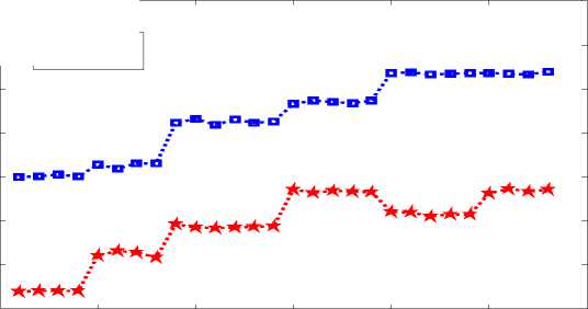
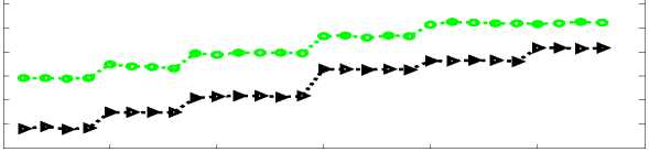
Figure 7 (a) shows the average energy consumed by the system when the LPU and the HPUs are learning. The LPU consumes less energy compared to the HPU. This should be expected because of the difference in their transmit powers. As the learning progress, the energy consumed is reducing. This is because the users are learning to use either the optimal bidding price to find out the appropriate number of users to be introduced into the system depending on the traffic load in the system.

While Fig. 7 (b) shows the utility based on the total energy consumed by the system (both HPU and the LPU) when all the users are learning and the average energy when one of the user is deviating from the learning model. It can be seen that the average energy consumed with one deviation is significantly higher. This is because when one of the players is not learning, the energy consumption level of the players is increased compared to when all the three players are learning. The learning process gets better for the learning players as the number of iteration increases and the amount of energy consumed reduces until the best utility is obtained.

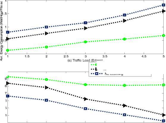
Figure 8(a) shows the average energy consumed per file sent against traffic load with all three players are learning, the average with one of the users deviating from the learning model and when none of the players are learning. It can be seen that as the traffic load increases, the energy consumption increases for all the scenarios. This is because as the traffic load increases the collision and activity in the system increases. When all the three players are learning the average energy consumption is lower and the reason is the same as explained for Fig. 7. It can be seen that using – 705 –

(a) Traffic Load (Erlang)

All Learning

Average With One deviation

No Learning

0.5

0.4

0.7

i ।

0.6

(b) Traffic Load (Erlang)

Fig. 7. The Average energy consumed by LPU and HPU (b) The Average energy consumed by all learning and average with one of the players deviating

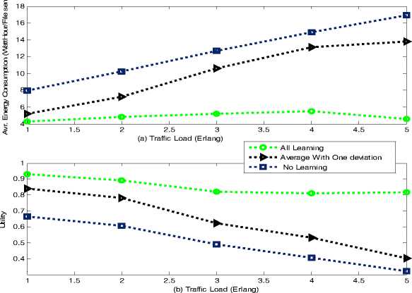
Fig. 8. (a) Energy Consumption (b) Utility in terms of energy consumption the proposed model an average of 40% of energy is saved compared to when none of the users are learning.

Figure 8(b) shows the utility obtained in terms of energy consumption ( U_E ) against traffic load. It can be seen that the average utility falls with the traffic load because as the traffic load increases the activity in the system increases and more collision occurs in the system. As expected when all the three players are learning, the average utility is significantly more than when a user is deviating especially – 706 –

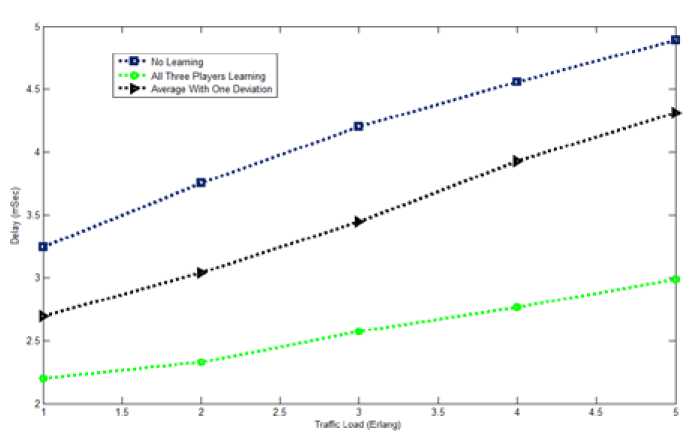
Fig. 9. The system delay with all three scenarios as the traffic load increases. At lower traffic load, the users can avoid each other by transmitting on different channels, making the values closer at lower traffic loads compared to higher traffic loads. It can also be seen that with the proposed model there is an average of 20% increases in utility compared to when the learning process is not used.

Delay is one of the important parameters that determine the functionality of a wireless network. This is because different applications have different tolerance level for delay. Hence the delay experience by the players is also examined. Fig. 9 shows the delay against the traffic load when all the players are learning, when one of the players is deviating and when all the players are deviating. The delay increases as the traffic load increases for all the 3 scenarios because as the traffic load increases, the number of users entering the system also increase, thereby, increasing the delay. It can be seen that the delay in the system is lower when all the players are learning compared to when one player is deviating or all are deviating. There is an average of 33% reduction in delay using the proposed model for all traffic loads that was considered.

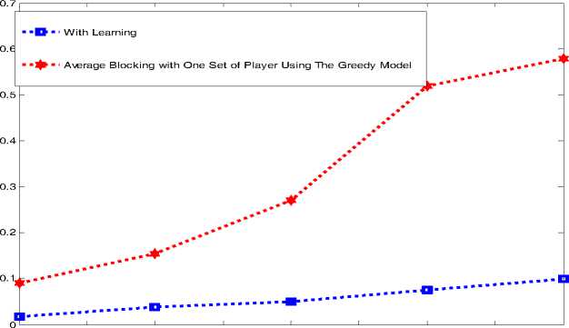
Another important performance metric in a wireless communication network is the blocking probability. Hence the blocking probability is examined to see if there is an improvement in the blocking probability of the system with the players learning. Fig. 10 shows the blocking probability of the system when all the three players are learning and the average blocking when one of the players is deviating from the learning model against the traffic load in the system. It can be seen that as the traffic load increases, the blocking also increases. This is because there is an increase in the system’s collision. This result shows that learning reduces the blocking experienced by the users. Hence, the performance parameters are better with learning.

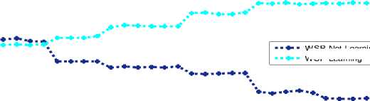
All the three players are contributing one way or the other to the performance of the system, hence the effects of the WSP not learning is examined. Fig. 11(a) shows the utility obtained by the WSP when learning and when using the greedy model. As expected, the utility obtained when learning is significantly higher than when not learning. This is because when the WSP is not learning, the reserve – 707 –

£

р

й

1.5

4.5

2.5          3          3.5

Traffic Load (Erlang)

Fig. 10. The blocking probability for all three players learning and the average with one of the three players deviating from learning

0.9

0.8

0.7

0.6

0.5

0.4

(a) Iteration

WSP Not Learning WSP Learning

0.8

0.4

4.5

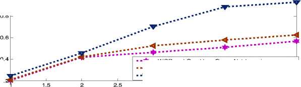
■*■ WSP and One User Group Not Learning

■<■ WSP Not Learning and Both User Group Learning

■▼■ All Three Players Learning

3          3.5

(b) Traffic Load (Erlang)

Fig. 11. (a) Utility against traffic load (a) WSP is learning at 3 Erlangs and WSP not learning (b) WSP and one of the users is not learning

price in the system is not set to reflect the present situation. Hence, the learning process does converge at a non-optimal value. This shows that it is important for the WSP to learn and use the reserve price to control the admission process. Fig. 11(b) shows the average utility obtained when the WSP and one of the users is not learning, when the WSP is learning but the other two players are not. For all three scenarios the utility obtained by the WSP increases. This is because as the traffic load increases, more of the available channels are in use. The results also show that the greater the number of players not learning, the lower the overall utility.

The results show that none of the players are better off or are having a higher utility value by deviating from the learning model. This shows that learning by all the three players forms a Nash Equilibrium for the proposed game model giving the definition of Nash equilibrium in [70].

• VI.    Conclusions and Future Work

This paper developed a learning scenario where all the users in the system can learn simultaneously. Different parameters were learnt by each of the users in the game model. Utility functions which were explicitly dependent on four parameters which determine the satisfaction received by the users was proposed. The utility function was based on the bid price, the green payments and the energy consumed by the user during the auction process. The results also showed that the energy consumed by the system is lower when all the users are learning the different parameters about each other compared to when of the player group is using the greedy model. As part of the future work a more mathematical model would be developed for the proposed system.