A generalization of Otsu method for linear separation of two unbalanced classes in document image binarization

There are many commonly used algorithms for image binarization [1] employed for various applications: digital documents compression [2], intelligent document recognition [3], medical image analysis [4], object detection [5, 6], digital image enhancement [7], porosity determination via computed tomography [8], forensic ballistics [9]. The diversification of methods is associated with the fact that the algorithm allowing for the equally high accuracy in all image processing tasks has not been developed yet. The efficiency of any chosen method depends on its statistical properties and constrictions.

Binarization methods can be classified according to the number of tuning parameters. The most convenient methods for users (i.e. for researchers engaged in the related fields or engineers) are the zero-parametric methods, which do not require the parameters tuning to match the expected properties of the input data. One of such methods is commonly used Otsu method [10], which automatically determines the optimal global threshold that separates pixels into two classes based on the intensity histogram. The simplest one-parametric method requires a user to set such threshold. Yet, in some cases, the global methods can demonstrate good results, and the corresponding conditions are of great interest.

Foundation for Basic Research No. 19-29-09066

The well-known Niblack's method [11] in its classical implementation has two tuning parameters, one of which is responsible for the window size and is regulated depending on the expected size of the segmented objects. The issue of the parameter adjustment for the certain application is not trivial and usually is resolved via the optimization on the subset of the available sample images, while some criterion of the binarization accuracy is selected [12].

Currently, the most accurate binarization methods are based on the artificial neural networks (ANNs) [13, 14]. Such networks employ a lot of tuning coefficients, the optimization of which requires many properly annotated pixel-precision examples of the classification. Despite this, the trained neural network is usually considered to be zero-parametric method suitable for employment by researchers or engineers with no machine learning experience. Nevertheless, this approach still requires a user to study the limits of the applicability of any chosen network, which could be nontrivial.

In this work, we consider document image binarization – the separation of two well-defined classes of pixels: contents of the document (pixels of printed or handwritten text lines, elements of the document structure, and other graphic primitives), and background regions which usually have uniform or weakly textured brightness pro- file. This problem is characterized by the unbalanced weights of these two classes of pixels, i.e. document image consists of mainly background rather than the contents. And a priori information about the document can significantly simplify the binarization. Thus, in many systems, prior to the binarization, the document type for each input image is being determined in order to select the appropriate binarization algorithm and its parameters, which helps to resolve the interpretation uncertainties of pixel groups in complex cases (e.g. [15]).

Unlike in automated identification document processing (where the templates are known beforehand), the preliminary document type categorization for hand-written and historical document image binarization is not feasible.

Because of the importance of this application, to track the developments in historical document binarization, a special competition Document Image Binarization Contest (DIBCO) has been regularly organized since 2009 [16]. To compare the proposed methods, the formal criteria for accuracy evaluation were established, but there are no restrictions on running time and memory consumption. Such conditions led to the dominance of the ANNs methods. Nevertheless, the fast binarization algorithms are becoming increasingly important, e.g. a new competition Document Image Binarization (DIB) [17] has been recently established, which judges algorithms not only by the accuracy, but also by the running time.

The winner of DIBCO 2017 is a neural network binarization method described in [18]. This method requires the scaling of an input image, and the optimal scaling coefficient depends on the size of the text symbol. Thus, the preliminary scaling coefficient is a hidden parameter of this method. In other similar works, such an analysis was not performed. But we can assume that similar methods require normalization of the input data. Given that, the number of normalization parameters should be considered to be the number of method parameters. Document images are not self-similar and their normalization usually includes scaling [19], thus the effect demonstrated in [18] could be expected.

It must be noted that the histogram-based methods, which include Otsu method, are scaling-invariant and do not require any additional preprocessing.

Thus, it is interesting to analyze the accuracy of the document image binarization employing one of the fastest methods – the zero-parametric Otsu method and its less known modification for cases where the weights of the classes to be separated are not considered equal [20]. We also consider the feasibility of the accuracy improvement for this algorithm employing an additional parameter of the scale of the images.

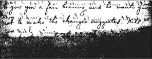
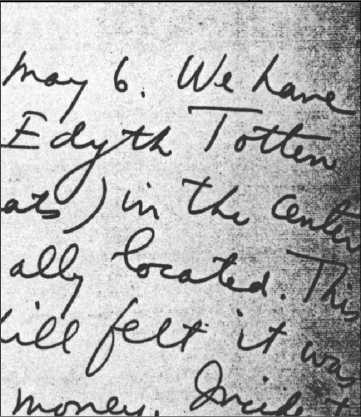
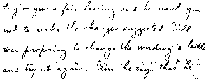
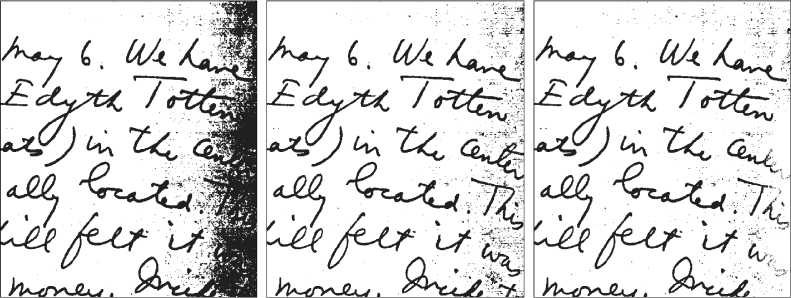
Further in this work, the known Otsu method modifications and the scope of its applicability are discussed. Pseudo F-Measure, the metric employed in DIBCO, is analyzed. We demonstrate that the unbalanced Otsu method modification [20] is better than the classical Otsu method by approximately 3 points in pseudo F-Measure metric. Also, we suggest a novel one-parametric (with window size as a parameter) generalization of Otsu method for two features using fast method of binary clustering [21]. The proposed method, which employs brightness average over window as the second feature, allows for the image binarization improvement of unevenly illuminated documents and documents with spots by 15 points. In Fig. 1, we illustrate the examples of the classical Otsu method, its unbalanced modification and the proposed one-parametric modification performance on the image from DIBCO dataset.

c)

a)

b)

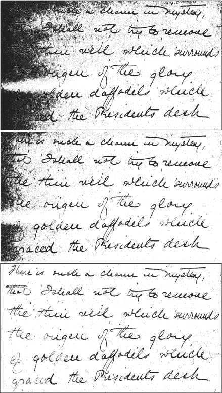
Fig. 1. The classical Otsu method (a), the unbalanced modification (b) and the proposed two-dimensional modification (c) performance on the hand-written document image

1.    An overview of the known Otsu method modifications

Suggested in 1979, Otsu method was one of the most frequently mentioned thresholding methods in 2004 [22]. To date, when comparing the binarization algorithms, Otsu method is often used as the baseline. It is also true for DIBCO. In most cases, Otsu method demonstrates quite low accuracy, although sometimes it is not significantly worse than the competing algorithms. For example, in 2016, the best algorithm was better than the classical Otsu method by 5 % [23], and in 2014, by 2% [24].

This can be associated with relative simplicity of the dataset (i.e. there were not many images with gradient illumination and overlapping distributions of background and text brightness).

To date, there are many known Otsu method modifications. The deviations involve the optimized criterion, search algorithms and even dimensionality of the analyzed feature space. Below we consider such modifications and their possible influence on the binarization accuracy in DIBCO.

Although there are many papers discussing Otsu method for various applications (the original paper on Otsu method was cited by approximately 32000 works in June 2019), there are not many works dedicated to its generalization. First, the paper by Kurita [20] should be acknowledged. It systematically describes the approach to the separability criterion search based on the maximum likelihood under assumption that the histogram is a mixture of two components, specifically, normal distributions. Three cases are considered: weights and components variances are equal (classical Otsu method), weights and components variances are arbitrary (the Kit-tler–Illingworth method [25]), and arbitrary weights while variances are equal (unbalanced Otsu method). It is worth mentioning that the classical Otsu method and the Kittler-Illingworth method are significantly more often featured in works than the unbalanced Otsu method, and thus, the first two are better studied than the latter. In particular, it is a widely known fact that the Kittler-Illingworth method is not stable (because it has too many degrees of freedom for a histogram-based method). To increase its robustness, in work [26], the authors suggested to introduce the restrictions for the target parameters.

The works by research group from King Saud University in Saudi Arabia should be also acknowledged. In [27], the authors suggested a separation criterion under the assumption that the mixture components follow lognormal distribution or Gamma distribution instead of the normal distribution. They demonstrated that under such assumptions the binarization accuracy could be increased, but the testing dataset was not large (only 13 images). In their other work [28], the authors proposed an approach to accelerate the classical Otsu method. They suggested to calculate the Otsu criterion only at local minima of the histogram, thus limiting the required computations. Prior to this work, the authors have published [29], which suggests the recursive binarization approach, where for the left part (in relation to the Otsu threshold) of the histogram the binarization threshold was calculated again in order to separate text from the complex background.

The development of Otsu method in certain cases allows for the binarization accuracy increase without involvement of the additional features. Nevertheless, there are certain effects, which are not compatible with any global threshold method. Let us consider the following list :

• 1.    non-uniform lighting;

• 2.    paper fold outlines;

• 3.    ink spots and stains;

• 4.    textured (“heraldic”) background;

• 5.    high level of noise.

2.    Test datasets and accuracy measure

Under any condition from this list, the brightness of some regions of the background may be lower than that of the symbols in other regions, and then the proper binarization via the global threshold is not feasible. In such cases, the local binarization methods are used. One of the most popular local binarization methods was proposed by Niblack [11]. It classifies pixels globally via certain threshold function, and not in one-dimensional brightness space, but in three-dimensional feature space “brightness – its average over window – its window variation”. Parameters of the classifier are not determined by the distribution in the image, but should be set beforehand, which makes this method unstable, i.e. vulnerable to changes in the external conditions. Otsu method does not have any limitations regarding the input histogram dimensionality, which theoretically allows for the employment of the same features, and for the automatic search of the classifier parameters. Mainly due to this fact, there are generalizations for Otsu method for two-dimensional and even three-dimensional histograms.

For the first time, such a generalization for Otsu method was described in [30]. The authors suggested the image binarization via the analysis of the twodimensional histogram, the first axis of which is the pixel brightness, and the second axis is the local average over window. Later in [31], Jian Gong et al. suggested the fast computation of the two-dimensional Otsu criterion described in [30] via cumulative summation: with cumulative histogram image computed once, it is feasible within the fixed timeframe to calculate weight (sum of all histogram pixels) of any orthotropic rectangle (which was used as the separating surface) with its vertex at the origin. This is also true for different statistics (mean, variance, and etc.). These statistics are further employed to calculate the criterion of the separation into two classes, rectangle and its complement, within the fixed timeframes. Later, in [32, 33] independently, there was suggested the same modification of the Jian Gong method: the criterion was calculated only via the most informative (according to the authors) part of the histogram. In 2016, in [34], it was demonstrated that the separation criterion calculation via two parameters (when the separating surface is a rectangle) can be performed independently via each parameter, which significantly reduces the computational time for the optimal separation without accuracy loss. Later, independently from the previous work, this approach was used in the paper dedicated to the development of the three-dimensional Otsu method [35].

Starting with Jian Gong’s research and later on, many authors work with rectangles, because the attempts to develop a fast brute-force search of the separating lines parameters failed, while lines are the optimal separation surfaces for equal covariance matrices in accordance with the original assumptions of Otsu method. An alternative two-dimensional histogram-based binarization approach is described in [36]. The authors suggested that the pixel brightness and the sample mean do not correlate, thus the pixels distribution on the two-dimensional histogram is stretched along the diagonal containing zero. Based on this observation, the computations acceleration was suggested: the one-dimensional binarization performed via the projection of the two-dimensional histogram onto the diagonal.

Besides the modifications approach, there are some papers which suggest acceleration of the Otsu criterion calculation based on the genetic optimization algorithms [37] and GPU-accelerated computations [38].

Currently, Otsu method and the Kittler–Illingworth method are more often employed as part of some combination of the methods. In particular, Otsu threshold is used as an input parameter during the pre-processing [39, 40], for the binarization of the “simple” images [15, 41– 43], and for global threshold value computation [44].

For this work, we selected 150 images from the following datasets:

• 1.    DIBCO Dataset (Document image binarization competition) [13, 16, 23,24].

• 2.    PHIBC Dataset (Persian heritage image binarization competition) [45].

• 3.    The Nabuco Dataset [46].

• 4.    LiveMemory Dataset [47].

The first three sets include images of the historical hand-written and printed documents with various distortions (inconsistent paper color, ink fading, blots, spots, seals, text showing through on the other side of the sheet, etc.). LiveMemory Dataset includes scanned proceedings of technical literature. Here, the main problems are symbols bleeding through on the other side and darkened paper fold outlines. It turned out that not all of the images from these datasets have pixelwise ground truth, and such images were not used. Thus, the compiled set included 150 images. Then it was separated into three subsets according to the image contents: 1) “simple” group includes 32 images; according to their annotation, they can be sufficiently (with accuracy over 95 %) binarized via global thresholding; 2) “complex” – the rest of the images; 3) “spots and shadows” – subgroup of “complex” group, which includes images with spots and shadows (21 images). The description of such a set and its separation is available at [48].

We evaluate the accuracy of the methods via one of DIBCO’s metrics. Let us describe it. In document image binarization, the recall is defined as the ratio of the number of pixels labeled correctly over all the possible correct pixels corresponding to the ground truth, including those that were not labeled right but that should be included in the result (false negatives). Precision is defined as the ratio of the number of all correct values retrieved over the total number of the values retrieved. F-Measure (harmon- ic mean of recall and precision) is commonly used to rank classification algorithms.

According to [49], F-measure is not a proper way to evaluate binarization quality, since it does not take into account the localization of the mislabeled pixel in relation to the document contents. For example, the loss of the symbol’s pixel is worse than the background pixel labeled as text. Thus, the author suggested the following modifications to the metric: pseudo-recall, pseudoprecision, and pseudo F-Measure.

Pseudo-recall is calculated as follows:

R ps

£ B ( x , y ) ■ G w ⁽ x , y )

■ £ G w ( x , У )

• x , y

  
  

where B ( x , y ) is a binary image, G w ( x , y ) is a segmented binary image multiplied with a weight mask. The latter is formed in a way that grants false negative pixels in text regions for an ideal result the lesser penalty the thicker the line width of the symbol is and the larger the distance from the border is. The weighted accuracy is defined as follows:

p ps

Z G ⁽ x , y ) ■ B w ⁽ x , y ) x , y

£ B w ( x , y )

• x , y

  
  

where G ( x , y ) is a segmented binary image, B w ( x , y ) = B ( x , y ) P w ( x , y ), and P w ( x , y ) is a weight mask tuning penalties for background false negatives based on the distance to a symbol. The goal of weighting is to increase the penalties for noise around a symbol and for the merged symbols. Thus, the pseudo F-Measure is defined as follows:

2 RP

___pS_pS_ ps psps

.

This metric is employed in DIBCO. We will use it further in this work.

Even though F ps became the standard approach to quality evaluation in document image binarization, this measure has certain drawbacks. In Fig. 2, we illustrate two images (possible binarization results) with different distortions, each featuring comparable numbers of black pixels. In the first image, there is a crossed-out piece of text, while its quality evaluation is F ps = 98.34. And in the second image, there is a thick horizontal line added onto the white background, and the quality evaluation is 97.22. Thus, according to F ps , it could be concluded that in some cases the information loss is not as important as the existence of the artifacts of the same scale. This is a very subtle effect, and it was not observed during the accuracy measurements of the considered methods on the selected set of images.

It is important to note that the structure of the Pseudo F-Measure is complex. The methods based on the ANNs can adapt to this measure and get the binarization accura- cy increase which will not reflect any real improvements. The “engineered” methods requiring fewer parameters (including Otsu method), on the contrary, cannot adapt to this metric, and thus, are less sensitive to its drawbacks.

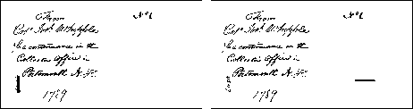
Fig. 2. The pair of the distorted images: the left image includes a crossed-out piece of text; the right image includes the black rectangle on the background

3.    One-dimensional criteria of Otsu binarization

In the original work [10], Otsu suggested the minimization of the between-class variance. The latter is defined as follows:

Q ( k ) =σ ² B ( k ) =ω 1 ( k ) ω 2 ( k )( µ 1 ( k ) -µ 2 ( k ))²,       (4)

where k is threshold level, and ω 1 , ω 2 , µ 1 , µ 2 are the weights and the sample means of the first and second classes respectively. One of the key results of [10] is the formula for the separability criterion: the author demonstrated that the separability criterion search can be described in only the first-order cumulative moments.

The separability criterion for the case when the populations of object and background classes are unbalanced was suggested in [20]:

Q ( k ) = ∑ ω i ( k )ln( ω i ( k )) - ln( σ w ) , (5) i = 1

where i is the index of the class, σ w is the within-class variance, which is defined as follows:

σ ² w = ∑ ω i ( k ) ⋅ σ i ². (6) i = 1

This criterion suits document images processing better, since the number of background pixels in document images almost always significantly surpasses the number of text pixels. This is confirmed by the experiments. For the entire selected dataset, the mean F ps was 87.57 for the unbalanced classes criterion, versus 84.3 for the classical one.

Tab. 1 demonstrates that the unbalanced Otsu method for all sets, except for the “simple” one, gives an average increase of 4%, and for the “simple” set the methods perform similarly. These results suggest that cancelling equal weight restriction for text and background classes allows for a higher binarization quality even for the complex images. Tab. 2 demonstrates two clear examples of the different results for binarization via classical and unbalanced criteria.

These results suggest that the further increase of the freedom degrees would allow for even higher binarization accuracy. However, on the contrary, the further generali- zation of the model (5) led to worse measure values: Fps for Kittler–Illingworth algorithm for the entire images set was 73.69, i.e. 10% less than for the classical Otsu method, and 13 % less, than for the unbalanced one. This is consistent with the previously reported results, in particular, with Haralick et al. findings [26].

Table 1. The comparison of classical and unbalanced Otsu criteria via F ps measure

	Classical Otsu, %	Unbalanced Otsu, %
Entire set	84.30	87.57
“Spots and shadows”	69.82	73.91
“Complex”	80.56	84.10
“Simple”	98.38	98.59

The maximum accuracy for the global threshold binarization methods for the entire set is 93.76. This value is a result of the optimal thresholds (for each image from the dataset) set via manual segmentation. It surpasses the balanced Otsu by 9.46, and the unbalanced by 6.19 percent points. Thus, for the test data, replacement of the balanced criterion with the unbalanced one is significant in terms of the accuracy, since it reduces the number of pixel classification errors by a factor of 1.5.

For further accuracy increase, there is a need for either new criteria of global threshold calculation, or for changes to the existing model. In the next section, we suggest the changes to the model, increasing the dimensionality of the problem, where the optimum threshold is computed via two features.

4.    The Otsu method for image binarization via two features

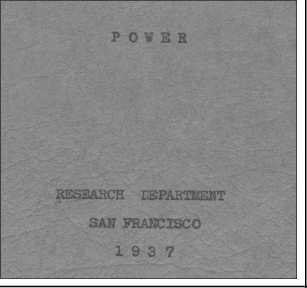
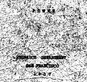
Let us consider the class of images, which incorporate spots or inhomogeneous background (sample images are illustrated in Fig. 3). Such images make up approximately 15 % of the considered set of images, which is significant. As shown in Section 3, utilization of both classical and unbalanced Otsu criteria for brightness histograms of such images results in unsatisfactory binarization accuracy (69.82 % and 73.91 % respectively). In this section, we suggest Otsu method for gray images binarization based on two features, allowing for successful binarization of the mentioned images.

Let us assign a two-dimensional vector to each pixel p of the image I to be binarized: v ( p )=< i , s >, where i is the intensity value of this pixel, and s is the local average intensity in the vicinity of δ , centered around p . Let us build the joint histogram H for the input image I based on the mentioned features. It can be considered as the digital image, where the vertical axis corresponds to i values, and horizontal axis corresponds to s values, and the intensity of the pixels corresponds to the number of vectors v =< i , s > in image I . Then the image binarization can be performed via the optimal separating surface in the joint histogram H image.

Table 2. The sample performance of the classical and the unbalanced Otsu methods

The input image

The classical Otsu criterion

The unbalanced Otsu criterion

d)

a)

b)

e)

a)

b)

Ogled po Gorenskem.

Poljanska dolina in pot skos njo proti Id

(Konec.)

Polagoma ее okrenemo okoli gricka ev. Antoni razgerne ее naeim ocein v deeni dolinici prijazno Idrija. Na konca gori ponosno etoji grajscFna, iz erede maii etolpicek v zrak moli; pod gradom pa i celi dolinici razprostira meeto , v kterega ВЧ^М^В

Fig. 3. Sample images featuring spots and inhomogeneous background

Let us consider two criteria for optimal separation of the histogram H into regions of two classes. These criteria, based on the maximum likelihood principle, are the generalization of one-dimensional unbalanced criterion for the case of two model features. The first of the latter is optimal for the unbalanced sets and covariation matrix with equal eigenvalues:

A ₁( θ ) = argmax ∑ ² ω _j ( θ )ln ω _j ( θ ) - ln( D ₁( θ ) + D ₂( θ )) ,   (7)

θ ∈ Ω j = 1

c)

f)

where Ω is the set of feasible separations in this model, θ are the parameters of a single separation option, ω j are the weights of the separated classes, and D j are the variances of their values. For the optimum second criterion, the covariation matrices of the mixture components without eigenvalues ratio restriction should be equal:

A ₂( θ ) = argmax ∑ ω _j ( θ )ln ω _j ( θ ) - lndet( ∑ S_j ( θ )) ,   (8)

^{θ ∈ Ω} j = 1 2           j = 1

where S j are the sample covariation matrices of each of the resulting classes.

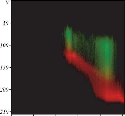
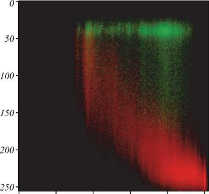
Fig. 4 illustrates the histograms for the images demonstrated in Fig. 3. They are visualized via three channel images, with red channel corresponding to the histogram of the background pixels, and green channel corresponding to the text pixels histogram. The cluster colors were obtained via segmentation. Fig. 4 a , b demonstrate that the background and text clusters are elongated. These figures also demonstrate that the assumptions of criterion (7) are not met. But there is no indication that the criterion (8) could perform better, since the distributions are not uniform and are not coaxial (fig. 4 b ). Thus, the criterion yielding the higher accuracy results can be determined only via computational experiments.

Let us consider different sets of feasible separations

Ω . For the global threshold segmentation based on the pixel intensity, set Ω I includes the segmentations via lines parallel to the x-axis and constructed by the only parameter θ = < I max >. Then the set of text pixels is defined as C T = { p ( i , s )| i ≥ I max }, and the set of background pixels is defined as C B = { p ( i , s )| i <  I max }. The listed examples show that a horizontal line cannot sufficiently divide text and background into two classes.

The set of the Jian Gong method segmentations is the set of all possible orthotropic rectangles (i.e. rectangles with sides, parallel to the coordinate axes) with one of the

vertices at the origin. These rectangles can be constructed via two parameters: q=< I max , S max >, where I max is the rectangle width, and S max is its height. After such separation, the following pixel set is assigned to the text class: C T = { p ( i , s )| i ≤ I max ∧ s ≤ S max }, and the following pixel set is assigned to the background class: C B = { p ( i , s )| i >  I max ∨ s >  S max }. Fig. 4 demonstrates that such separation would result in classification errors.

Let us consider set Ω L , containing lines, crossing the two-dimensional histogram. These lines can be set via two

Brightness

О 50      100     150     200 . 250

a)                            Average over window

Fig. 4. The histograms of images illustrated in fig. 3

Step 1 : For the input image I with sides w and h , the histogram H is built based on the features v =< i , s >. The feature s is calculated via squared window with the side of δ = 0,1 ⋅ min ( w , h ). The number of the histogram bins is 256 for each axis.

Step 2 : The criterion A is calculated via linear binarization clustering adopted from [21], and the parameters of the separating line <  k , i 0 > are defined (the detailed description and pseudocode are given in [21]). It is worth to mention that linear binarization clustering method utilize fast Hough transform algorithm, which has wide range of application, such as [50]. The considered set of the separating lines is limited in the way that assures an angle between each line and the horizontal axis is less than 30 degrees. This allows for a higher algorithm performance.

Step 3 : For each pixel p ∈ I , the vector of features v ( p ) is calculated. Based on the computed parameters <  k , i 0 > of the line, p is assigned to either background class or text class according to the rule above.

It must be noted that in Step 1 the choice of the histogram binning scale is not specified: there can be used either the scale of absolute values or the range between minimum and maximum calculated features. For criteria A 1 and A 2 , the choice of the scale affects binarization accuracy differently. The results reflect the accuracy for A 1 in terms of the scale with absolute values, and for A 2 in terms of the range, calculated via features values.

parameters: θ =< k , i 0 >. Then the background class consists of the pixel set C B = { p ( i , s )| i ≥ ks + i 0 }, and the text class consists of C T = { p ( i , s )| i <  ks + i 0 }. The figures show that for two-dimensional histograms, there could be such slant lines selection, which would allow for good segmentation.

In [21], the algorithm for fast computation of (7) and (9) criteria on Ω L segmentation set was suggested. Let us adopt it for the image binarization algorithm. The inputs of the algorithm are: the gray image I , and separation criterion A . The algorithm includes the following steps:

Brightness

0      50     100     150     200    250

b)                            Average over window

Let us evaluate the complexity of the suggested algorithm. The computations of Step 1 and Step 3 require O ( n , m ), where n and m are the linear size parameters of the image. The complexity of Step 2 depends of the histogram size. Employing the method, suggested in [21], the complexity of the binarization criterion computation for all lines and its optimal value search is O ( h ² log h ), where h is linear size of the histogram (as previously mentioned, h = 256). Thus, the total complexity is O ( h ² ln h + nm ), which is comparable with Jian Gong algorithm complexity – O ( h ² + nm ) [31].

Fig. 5 demonstrates performance results on the images with complex background of the suggested algorithm for criteria A 1 and A 2 , and of the one-dimensional algorithm for the unbalanced criterion.

Tab. 3–5 demonstrate the results of the onedimensional Otsu method for the unbalanced criterion, and of the proposed Otsu method for two-dimensional histogram for criteria A 1 and A 2 .

Tab. 3 shows that for the entire set, A 1 works the best. This fact suggests that the employment of the average over window as the additional feature allows for a higher binarization accuracy of the global threshold function (line) in two-dimensional feature space “brightness – its average over window”. Tab. 4 shows that all three binarization methods grant similarly accurate results for the “simple” images set.

Table 3. F ps values for the entire set of images
	Mean	Median	Variance
Unbalanced Otsu	87.57	91.98	14.03
Criterion	91.22	93.90	10.35
Criterion	89.63	93.53	13.61

Table 4. F ps values for “simple” set of images

	Mean	Median	Variance
Unbalanced Otsu	98.59	98.64	0.91
Criterion A 1	98.64	98.64	0.90
Criterion A 2	98.55	98.51	0.74

a)

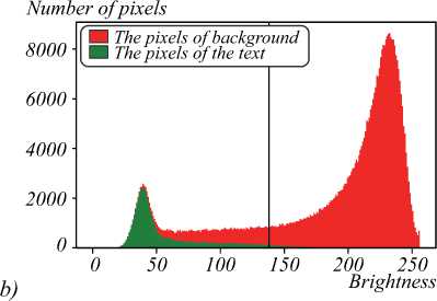
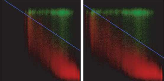
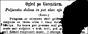
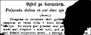
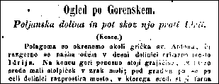
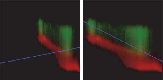
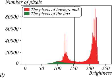
Fig. 5. The binarization algorithms performance results. The first column in a) and c) panels demonstrates the image binarization

results by Otsu method with the unbalanced criterion; b) and d) panels demonstrate histograms and binarization threshold for a) and c) respectively. Similarly, results for two-dimensional modification of the method with criterion A 1 in the second column, and criterion A 2 in the third column, are presented

Tab. 5 details the binarization accuracy on “spots and shadows” dataset. It shows that no matter which criterion is used, two-dimensional method is more accurate. It is worth mentioning that the criterion A 2 is better for the image binarization of documents with uneven illumination or spots.

Table 5. F ps values for “spots and shadows” set of images

	Mean	Median	Variance
Unbalanced Otsu	73.91	77.17	18.84
Criterion A 1	84.06	88.85	17.26
Criterion A 2	89.64	90.12	6.02

Conclusion

This work considers document image binarization via Otsu method with classical (balanced) and unbalanced criteria. Pseudo F-Measure on the set of 150 test images showed that the accuracy of these methods was 84.3 % and 87.57% respectively (the maximum Pseudo F-Mea-sure value of this global binarization model was 93.76%). We demonstrated that for document image binarization the lesser-known Otsu method with unbalanced criterion allows for a higher binarization accuracy. The international document binarization competitions in certain years (when the dataset was suitable for global binarization) showed that one-dimensional Otsu method with unbalanced criterion was comparable with the best competing algorithms in terms of the accuracy, which confirms Otsu method practical importance.

This work also demonstrates new generalization results for Otsu method in image binarization via two features. The proposed algorithm employs fast linear clustering of two-dimensional histogram for search of the parameters of the line separating background and text pixels on this histogram. We demonstrated that for many cases (if image includes inhomogeneous background or spots), the slant line is the optimal separating surface for twodimensional histogram. Computational experiments for test datasets showed that Otsu method with two features employing the considered criteria allowed for average accuracy of 89.63 % and 91.22 % respectively.