A Genetic Algorithm Inspired Load Balancing Protocol for Congestion Control in Wireless Sensor Networks using Trust Based Routing Framework (GACCTR)
")
Author: Arnab Raha, Mrinal Kanti Naskar, Avishek Paul, Arpita Chakraborty, Anupam Karmakar
Journal: International Journal of Computer Network and Information Security(IJCNIS) @ijcnis
Article in issue: 9 vol.5, 2013.
Free access
Wireless Sensors Networks are extremely densely populated and have to handle large bursts of data during emergency or high activity periods giving rise to congestion which may disrupt normal operation. Our paper proposes a new congestion control protocol for balanced distribution of traffic among the different paths existing between the Source node and the Sink node in accordance to the different route trust values. This probabilistic method of data transmission through the various alternate routes can be appropriately modeled with the help of Genetic Algorithms. Our protocol is mainly targeted in selecting the reliable or trustworthy routes more frequently than the unreliable ones. In addition, it also prevents concentration of the entire data traffic through a single route eliminating any possible occurrence of bottleneck. The merits of our protocol in comparison to the presently existing routing protocols are justified through the simulation results obtained which show improvements in both the percentage ratio of successful transmission of data packets to the total number of data packets sent and the overall network lifetime.
Load balancing, Genetic Algorithms, Direct Trust, Route Trust, Network Lifetime
Short address: https://sciup.org/15011223
IDR: 15011223
Text of the scientific article A Genetic Algorithm Inspired Load Balancing Protocol for Congestion Control in Wireless Sensor Networks using Trust Based Routing Framework (GACCTR)
Wireless Sensor Networks can be appropriately defined as a collection of spatially and temporally distributed/used sensors i.e., devices that are capable of interacting with the environment either by sensing or controlling physical parameters. WSNs, which have been till recent years primarily a subject of only research interest, nowadays, are increasingly finding widespread use in industry for various monitoring, alerting, data gathering and surveillance applications. This is mainly due to the inherent advantages that WSNs provide to the consumers like easy deployment, programmability and re-programmability, self-configurability and their multifaceted applications. However, WSNs are largely constrained in terms of hardware specifications, processing capability, energy availability and maintainability.
Congestion Control (CC) and Congestion Avoidance (CA) are two of the most desirable qualities required for the proper functioning of a Wireless Sensor Network (WSN). Congestion in WSN results from large amount of data transmission throughout the network. In a densely distributed WSN, a large number of nodes usually exists which provide many alternative paths or routes between a particular source and a particular sink. Appropriate choices of routes at various instants of time become an important necessity for congestion avoidance. The entire data is divided into a number of packets which are then distributed among the different routes by the source node and are accumulated and re-organized at the destination. The efficient routing of data through the available paths is very essential for both accurate data communication and lifetime enhancement – a vital requirement for the energy constrained WSNs.
Trust Management systems in Wireless Sensor Networks are increasingly becoming essential from the reliability aspect. Even in engineering, the meaning of Trust is not entirely different from its literal meaning. It is attributed to the opinion that one entity (or in WSN one sensor node) forms about a second exactly similar entity (again another sensor node). Depending upon the value of Trust (or in some cases Level of Trust), a particular node can be considered to be either Malicious or Benevolent. Malicious nodes usually affect the normal operation of the sensor network adversely such as by injecting duplicate packets, forwarding modified or distorted packets, sensing and sending wrong data etc. Due to these malicious nodes, sometimes most of the data and control packets get forwarded through a specified node or nodes causing enormous congestion and ultimately disintegration of the WSN. Sometimes, the nodes may even process data arbitrarily and can try to communicate with other nodes continuously as long as their batteries are not completely depleted. Presence of a large number of malicious nodes make the WSN prone to various types of attacks like Wormhole, Sybil, Sinkhole, Denial of message and HELLO flood attacks. Other variants of attacks are tampering, jamming, collision, desynchronization, traffic analysis and eavesdropping.
Wireless sensor nodes are increasingly being used for a variety of applications. In most of the cases, WSNs are highly populated and it becomes extremely difficult to monitor the performance of each and every individual nodes. Hence it becomes imperative to introduce energy aware as well as reliable routing protocols with an additional characteristic of sharing the traffic among the different reliable paths. So it can be rightly concluded that congestion control and trust based routing are actually interlinked as both have a mutual interdependence.
In this paper we propose a new Genetic Algorithm inspired load balancing protocol for Congestion Control in WSNs using Trust based Routing framework or GACCTR. It utilizes the core concepts and fundamental advantages given by GAs for distributing the traffic on the basis of reliability of the nodes. Simplicity and easy implementation are the main factors of selecting GA. As expected, the results show marked improvements in various network characteristics and properties over the existing protocols as mentioned in Section V.
The rest of the paper is organized as follows: Section II provides an account of some existing literature related to the proposed work. Section III gives the problem statement along with the major concepts used in developing our protocol. It also contains the proposed work given in the form a main procedure and its associated functions in the form of algorithms. Section IV and Section V present the simulation results and the conclusion respectively
II. RELATED WORKS
Trust based congestion control in WSNs is a new concept and has not been reported in literature to a great extent. However, some works based on traditional approach of congestion control for WSNs are found. Wan et al. propose CODA [1], a congestion detection and avoidance method for sensor networks in which open loop hop by hop back pressure and closed loop multisource regulation are used. CODA detects congestion by periodically sampling the channel load and current buffer occupancy. In [2], Hull et al. integrate three complimentary congestion control strategies that span different layers of the traditional protocol stack: hop by hop flow control, rate limiting and a prioritized MAC protocol. In ESRT [3], Event-to-Sink Reliable Transport protocol, both congestion detection and reliability level are estimated at the sink. ESRT places interest on events, not on individual pieces of data. Detection of events is related to the number of packets received during a specific interval. Sensor nodes must listen to sink broadcast at the end of each decision interval and updated their reporting rates. They monitor their buffer queues and inform the sink if overflow occurs. The major limitations of ESRT are only single hop operation support and pushing all complexity to the sink. The key ideas of another protocol PSFQ [4] are slow down distribution (Pump Slowly) and quick error recovery (Fetch Quickly) to avoid congestion. The drawback of PSFQ includes several timers setting, highly specialized parameter tuning and complicated internal operations.
All the above works do not consider the presence of malicious nodes in the network. The inexpensive sensor nodes are typically prone to failure. These malfunctioning nodes in the network increase transit traffic and latency by diffusing useless packets. Trust based approach eliminates the malicious nodes from the routing path and thereby reduce the network congestion. Although implementation of trust concept in WSNs is new idea, some research papers are available for trust estimation of sensor nodes and thus computing the most trusted routing path. In ATSR [5], routing decisions are taken based on geographical information as well as Total Trust (TT) value of the nodes. TT of a node is calculated by combining Direct Trust (DT) and Indirect Trust (IT) information of that particular node. In GMTMS [6], trust values of individual nodes are estimated by geometric mean of all relevant trust metrics. This model has certain advantage over Momani’s model [7], in which trust is calculated as arithmetic sum of different parametric probabilities and may lead to serious false value. Suppose, all parameters give high trust values except only one parameter, say successful packet transmission or packet latency. As per Momani’s model, a high trust value will be assigned even though packet transmission is zero or packet latency is infinite. This can be avoided in GMTMS by considering product or the geometric mean of the trust value of all parameters. In DTLSRP [8] protocol, Total Direct Trust (TDT) value is computed by GMTMS method. The nodes having TDT higher than a predefined application based threshold value can only participate in routing path. Link State Routing Protocol is used in DTLSRP to find out all available paths. The multiplicative route trust is computed for each path and highest route trust value is chosen as best routing path. DTLSRP performs better than other protocols like ATSR etc. However it does not include the Indirect Trust (IT) that is obtained from the feedback of neighboring nodes. TILSRP [9] protocol uses both DT and IT for estimating the trust value of sensor nodes. It uses LSRP based on trust and finds the best trustworthy route.
In FCC protocol [10], Zarei et al. propose a Fuzzy based trust estimation for congestion control in WSNs. The malfunctioning nodes are detected and isolated from routing path using fuzzy based trust estimation of the nodes. The resulting effects are some decrease in packet drop ratio and accordingly increase in packet delivery rate. FCCTF [11] protocol is modified form of FCC, in which the Threshold Trust Value (TTH) decision making is based on corresponding traffic ratio of the related region. TTH could change dynamically with increasing or decreasing form of traffic ration. By increasing TTH, more malicious nodes are detected and blocked and consequently useless packets are replaced by useful packets. Although FCCTF algorithm shows some improvement over FCC, still there is further scope of improvement in terms of congestion detection and control.
The fundamental theories and concepts of Genetic Algorithms as described in this paper have been taken from [12]. We also surveyed some already present WSN routing protocols based on Genetic Algorithms, however none were found based upon the Trust values of the nodes. For example, [13] proposes a new routing protocol GROUP which increases the network lifetime from the previously existing schemes of PEGASIS and LEACH by ensuring a sub-optimal energy dissipation of the individual nodes based on the principles of Genetic Algorithms along with Simulated Annealing. A GA based shortest path algorithm replacing the famous Dijkstra’s algorithm is described in [14]. [15] describes another GA based congestion controlling algorithm depending upon the different traffic rates handled by the sensor nodes within the sensor network.
III. THE PROPOSED GACCTR PROTOCOL
An excellent method to control congestion in Wireless Sensor Networks is through traffic balancing i.e. sharing of traffic among the different possible routing paths existing between the Source and the Sink. In this case ‘Traffic’ refers to the data or more specifically data sensed by the sensors of the WSN that needs to be communicated to the destination node.
The main difficulty in selecting a particular route for transmission of data from Source to Sink lies in the fact that the entire load gets concentrated on a single link. This means that while some nodes are active during the entire data sensing and sending duration, some other nodes remain completely idle. As a result both the lifetime and traffic handling capacity of the link diminishes significantly with time. One of the major disadvantages in using the protocol given in [8] for selection of the route is that it results in continuous switching of routing paths to send data from Source to Sink demanding greater processing capability and better congestion control schemes deployed throughout the Wireless Sensor Network.
The selection of the path can be precisely modeled with the help of genetic algorithms giving appropriate probabilities for selection of routing paths using the concept of Route Trusts [8], [9]. It must also be noted that in Genetic Algorithms, we can work with a concise and effective population of individuals that allow us to select the more trusted paths even at the inception of the network and hence makes the entire network more reliable for communication.
For implementing GACCTR, we have to first apply the Link State Routing Protocol or LSRP for finding out the routes between each pair of nodes. Routing tables are formed for each of the sensor nodes on application of this LSRP. As a result, a particular sensor node has the knowledge of all the routes by which it can communicate data to the destination node. Usually, for a densely populated wireless sensor network, a large number of paths exist between two nodes. However as a result of heterogeneous active durations of different sensor nodes due to some of them devoting relatively more time in sensing and communicating data compared to others, the residual energy (the remaining battery life) of the nodes are different.
Another important point that can be pointed out is that no network is completely isolated from external intrusions or sensor node malfunctioning. Some of the routes deciphered at the inception of the network gradually become unreliable with time either due to improper working of the nodes or due to low packet transmission rate. Reduced battery life also decreases the overall lifetime of the sensor network. As a solution, different methods are employed for uniform consumption of energy at different points of the network in order to enhance the overall lifetime of the WSN. GACCTR provides a set of routes having high fitness function values for distributing the load among the different paths thus helping in the homogeneous power consumption throughout the network. Now, we give a brief overview of the two most important tools used in GACCTR.
-
A. Genetic Algorithms
Genetic Algorithms (GA) are basically probabilistic search algorithms and optimization techniques based on the mechanisms of natural selection and evolution. They combine survival of the fittest among string structures with a structured yet randomized information exchange to form a search algorithm with some of the innovative flair of human search. A genetic algorithm maintains a population of coded forms of possible solutions of the problem of interest. In the language of GA, these coded forms are known as chromosomes. In most cases binary coding is preferred for easy manipulation and operation. Each chromosome is evaluated by a function known as the fitness function which is usually called the cost function or the objective function of the corresponding search or optimization problem. At first, the initial population is randomly generated. New populations are created in subsequent generations through the four fundamental mechanisms: selection, crossover, repair and mutation operations. Selection mechanism selects fitter individuals (parents) for crossover and mutation. Crossover is another important technique that causes the exchange of genetic materials between parents to produce offspring, whereas mutation incorporates new genetic traits in the offspring.
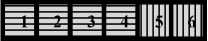
1 2 3 4 5 6


+
(a)
+
1 2 3 4 5 6
mean those nodes which can communicate directly with the concerned sensor node. We evaluate the Direct Trust with the help of the procedure given in [6].
As explored in [6], the DT is calculated as the Geometric Mean of the different Trust Metrics i.e. parameters and network properties. In implementing this protocol, the Trust Metrics used are shown in the following table:
Table 1: Trust Metrics used for implementation
% Successful Transmission of Data Packets/Messages
% Successful Transmission of Control Packets/Messages
Communication range normalized to the maximum communication range of all the sensor nodes within the WSN
II 1III2III3
(b)
+
(c)
+
(d)
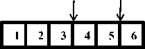

Figure 1. (a) Parents for one-point crossover; (b) Off-springs after one-point crossover; (c) Parents for two-point crossover; (b)
Off-springs after two-point crossover
Sensing range normalized to the maximum sensing range of all the sensor nodes within the WSN
Health (or Remaining Battery life)
The Direct Trust of node j with respect to its one-hop neighbor i is represented as T i,j . This convention is followed throughout our entire paper.

T i,j

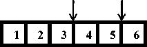
In Figure 1 and Figure 2 the chromosomes representing the parents and the off-springs are of length 6. The points of crossover are shown by arrows. Similarly in the figure below the mutation point is also shown with the help of an arrow.
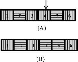
Figure 2. (A) Selected chromosome for mutation; (B) Offspring
-
B. Trust Based Routing Framework
In Wireless Sensor Networks, the technical meaning of the term Trust is the opinion a particular sensor node possesses about another sensor node. It is actually a probability which splits the sensor nodes into two categories: benevolent and malicious. This demarcation is based upon the Trust Threshold (TTH) value usually taken to be 0.50 by default. Usually trust of a sensor node can be defined in two ways: Direct Trust and Indirect Trust [7], [9]. In our protocol, we are only interested in the Direct Trust of the sensor nodes i.e. the opinion of sensor nodes with respect to its direct one-hop neighbor. By the term one-hop neighbors of a sensor node, we
Figure 3. Direct Trust of a sensor node j with respect to i
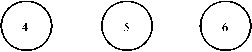
Now, usually a routing path consists of a large number of nodes starting from the Source and terminating in the Sink. For example, we take a routing path as follows:

Figure 4. A routing path with sensor node “a” and “g” as Sink and Source respectively.
Here, there are seven sensor nodes represented by the English alphabets a, b, c, d, e, f and g. Now as per our definition the Direct Trust (DT) of b with respect to a is given as Ta, b . Similarly the DT of c with respect to b is given as T b,c and it follows similarly. An expression which utilizes Direct Trust values to depict the reliability of an entire routing path is known as the Route Trust [8] and is represented here as RTγ, where γ is the path index. Now, the value of RT for a path e.g. the one given in Figure 4 is given as a product of the individual direct trusts of the consecutive sensor nodes belonging to the path with respect to its immediate preceding route in the path.
So, RT path given in Figure 4 = T a,b *T b,c *T c,d *T d,e *T e,f *T f,g . It is to be noted that we do not need to calculate the DT of the Source node with respect to any other node.
Suppose any two consecutive nodes of an arbitrary route κ are denoted by indices i and j. Let the total number of sensor nodes in the path is NS, then rTk = П£1"%+1 .......(i)
As evident in [8] and [9] the values of RTs are an indication of the route’s reliability i.e. greater the value of RT, more reliable a path is. In case of equal direct trust values, which is an ideal case – a situation that can be thought of at the time of first deployment of the WSN, the values of RTs also signify the shortest route between a unique pair of sensor nodes as proved in [8]. This also renders the application of Dijkstra’s algorithm to be redundant.
In [9] we have eliminated the malicious nodes from participating in routing before implementing the respective protocols. Although this results in making the routing process simpler, it also introduces additional overhead due to the protocol being a four step process.
Step I: Application of LSRP to decipher the possible routes from a definite Source to a definite Sink.
Step II: Calculation of individual Direct or Indirect Trusts.
Step III: Elimination of the malicious nodes from participating in routing.
Step IV: Calculation of the Route Trusts for the different routes as found out in Step I.
-
C. Main Procedure
Equation (i) has been adopted as the fitness function in this case. This function incorporates the Direct Trust (DT) values of the sensor nodes with respect to the preceding node belonging to the different routing paths. The calculated numerical value of the fitness function determines the route through which the data is transmitted from the Source to the Sink. This route actually signifies the most reliable or trusted path. The selection of the route being a probabilistic process, the path of data transmission is not fixed. Moreover the DT of a node being evaluated dynamically and updated periodically itself helps in balancing the load. Genetic Algorithms provide the most suitable way in this probabilistic modeling. The primary advantage of using GA is that it helps to identify the best routing path in reduced number of steps and duration. In addition to this quick convergence to the most appropriate path, GAs are also easy to implement and requires mediocre processing capability of the sensor nodes.
For practical implementation of the GACCTR we consider that all the sensor nodes have prior knowledge of their corresponding routing tables ie the routes existing between the node itself and all other nodes within the WSN. This assumption is valid since we have stated earlier in our work that the underlying basic routing protocol we use is Link State Routing Protocol (LSRP). However, the requirement of Dijkstra’s Algorithm for finding the shortest route from Source to Sink is redundant in our proposed protocol. The main reason for this is because our target is to choose the most trusted route instead of the shortest one. It can be shown also that in case the DTs of all the nodes are equal with respect to the one-hop neighbours, then the path that is chosen to route data, according to our protocol, is the shortest route possible from the source node to the destination one. This is also derived in [8].
C.1 Chromosome and its constituent genes: The fundamental step in GA is the evaluation of the fitness function which is represented as a function of the representative genes of the chromosomes. For our GACCTR, the chromosome denotes the routing path. The constituent genes depict the sensor nodes within the path and the gene indices G_0,G_1,…G_n etc., show the position of the sensor nodes starting from the Source node ie the node id stored in G_0 represents the source node or the node from where the data is generated. G_1 represents the next node after the Source node to which the data is communicated directly. Similarly G_i represents the ith node in the routing chain. The chromosome size L (or the number of genes) represent the maximum length of the route in terms of the number of nodes existing. Since, wireless sensor networks are extremely densely deployed; there exists innumerable paths between the initiating node and the terminal one. So it becomes imperative to impose an upper limit on the maximum length of the chromosome with the minimum being a direct connection between Source and Sink. It is evident that the length of the route will never be uniform. Hence to keep the length of the chromosome constant the non-exiting gene indices are padded with zeros.
G_0 G_1 G_2 ........ G_i G_L-1
Figure 5. An L length chromosome
|
a |
b c d e |
f |
g |
0 |
0 |
0 |
0 |
0 |
Figure 6. A 12-length chromosome representing the routing path in Figure 4
As mentioned earlier, equation (i) is also the fitness in this case. It can be restated in terms of sensor nodes represented as genes in Section C. 1 as f = RTi = Ш-о2^j,G_i+1 ........(ii), having a fixed
Source and Sink.
Application of the usual GA operators for initial population generation and subsequent generations through parent selection, crossover, and mutation as described in Algorithms 1, 2, 3, 4 and 5 respectively, help us to produce fitter generations of chromosomes subsequently representing more reliable routing paths. At some suitable generation, the fitness values are plotted for a Roulette Wheel Selection or Fitness Proportionate Selection [12]. In fitness proportionate selection [12], the fitness value is used to associate a probability of selection with each individual chromosome representing a routing path in our case. If f i is the fitness of individual i in the population, the probability of being selected is
Pi = —яД—........... (iii), where N„ is the number of
^j^fj p individuals in the population.
It is to be noted in this case that closer values of fis (or RTs in this case) render equal probabilities of route selection. The justification of the roulette wheel analogy can be envisaged by imagining a roulette wheel in which a candidate solution represents a pocket on the wheel; the sizes of the pockets are proportionate to the probability of selection of the solution. Selecting M chromosomes from the population is equivalent to playing M games on the roulette wheel, as each candidate is drawn independently [16]. So, it is evident from utilization of this rule that no route is fixed from transmission of packets from the Source to the Sink. The method being completely random helps us in distributing the load among the different routing paths, with GA helping in finding the more reliable ones.
Algorithm1. Initial Population Generation Algorithm
Inputs: g <= Initial population size i .e. number of individuals in a generation;
N <= Number of nodes in the WSN
So <= Source Node
Si<= Sink Node
D <= Routing tables along with Route Trust (RT) values available in each of the nodes present in the WSN
Output: Set of routing paths from a particular Source to a particular Sink
Proc edure generate_initial_population();
temp2 = So
Loop1: for j=1:g
Set trust values of nodes once crossed to zero in data table
Loop2: for i=1:N m=1;
Loo p3: for k=1:N if(data1(temp2,k) > 0
p2(m) = k; % storing the node values that can be trusted in array p2
m=m+1; %incrementing the counter end Loo p3
ran_num=randi(length(p2)); % generating random number of length of array p2
temp 1 = p2(ran_num); % storing element from p2 in temp1
If (temp2 is equal to Si)
Terminate loop2
Endif
If (Si not reached within N repetitions)
Set generation to zero and start over loop2
End if
End loop2
temp2=So; % setting temp node to source node value for next generation starting data1=data; % reload trust value chart
End Loop 1
Display initially generated population
End Procedure
Algorithm 2. Parent Selection Algorithm
Inputs : population ,N( no. of nodes)
Outputs: selected_pop,trustofpopulation(w)
Procedure Selection();
L= no. of members in population for j=1:L for i=1:(N-1)
temp 1=population(j,i) ; /*Store first node in temp 1*/ temp2=population(j,(i+1)); /*store second node in temp2*/ if(temp2 < 0.01) /* if destination node value is zero break*/ break;
endif
w(j) = w(j)*data(temp 1,temp2); /* product of trust values of each path stored in weight matrix*/ endfor for i =1:L
r(i) = w(i) + prev; /* adding the previous value of weights to obtain a continuous range from 0 to 1*/ prev = prev + w(i);
end end
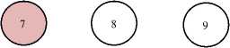
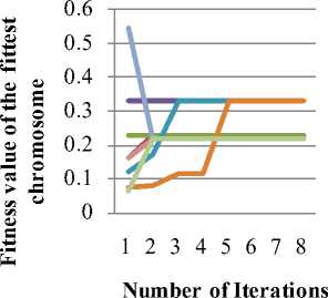
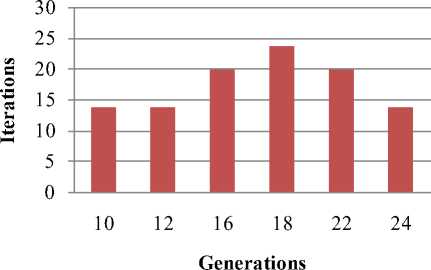
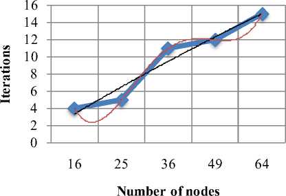
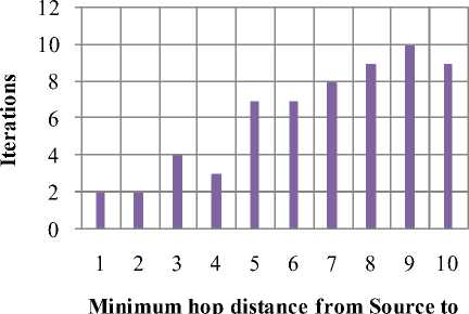
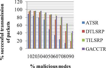
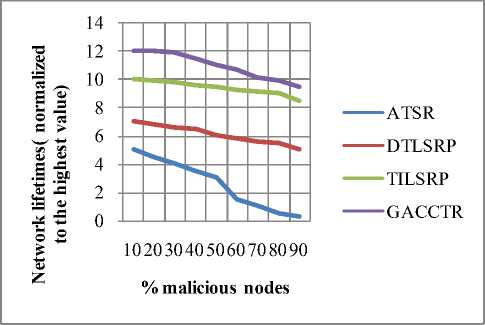
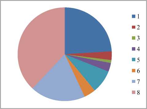
Display pie diagram /*displays the equivalent roulette wheel*/ for i=1:L if( r(i) < roll break; endif endfor for i=1:l selected_pop(i,:) = population(selected(i),:); /*selected population*/ end Endfor End Procedure An important assumption from the point of implementation of GACCTR is that we have assumed only One-Point Crossover here for simplicity. It is to be noted that two-point crossover could have also been done but then we would have to compromise processing complexity with that of flexibility. It has been however found as shown in Section IV, that our GACCTR performs very efficiently with the one-point crossover scheme. Algorithm 3. One-point Crossover Algorithm Inputs : Selectedpop , no. of nodes Outputs : Crossoverpop Procedure Crossover(); L = no. of members in population For i=1:2: L a= number of non-zero element in first parent b= number of non-zero element in second parent crossover point = ceil((a+b)/4) /* Round off the crossover point to nearest integer if it’s a fraction*/ for j=1:crossover point tempstore(j) = firstmate(1,j); /* store the elements of first parent from starting to crossover point in temp matix*/ endfor for j=1:crossover point firstmate(1,j) = secondmate(1,j); % rewrite the elements of first parent from start to crossover point with elements of second matrix secondmate(1,j) = tempstore(j); % rewrite elements of second matrix with that of temp matrix endfor Send paths for repairing to ‘Repair’ Program newgen(i,:) = firstmate(1,:); newgen((i+1),:) = secondmate(1,:); newgenfit = fitness of crossover generation parentfit = fitness of parent generation for j=1:2:L temp(1) = newgenfit(j) temp(2) = newgenfit((j+1)) /*store the fitness value of new generation of the two offsprings*/ temp(3) = parentfit(j,:) /* store the fitness value of parentgen*/ temp(4) = parentfit((j+1).:) tempgen(1,:) = newgen(j,:); /* store the offspring node path*/ tempgen(2,:) = newgen((j+1),:); tempgen(3,:) = selected_pop(j,:); /* store the parent node path*/ tempgen(4,:) = selected_pop((j+1),:); [~, i1] = max(temp); /* obtain the index position of the path having greatest trust value */ temp(i1) = 0; /* set the trust value of the path having highest fitness to zero*/ [~, i2] = max(temp); /* obtain the index position of path having next best fitness*/ finalgen(j,:) = tempgen(i1,:); /* store the path having highest fitness*/ finalgen((j+1),:) = tempgen(i2,:); /*store the path having next best fitness*/ Endfor End Procedure Algorithm 4. Repair Algorithm Inputs: row_mat Outputs : repaired_mat Procedure Repair(); N1 = index position of last non-zero element N= number of nodes Data = matrix containing trust values For i=1:N1 Element = row_mat(:,j) Comparison = find(row_mat==element) If(length(comparion) > 1) Firstindex = Comparison(1); Lastindex = Comparison(2); For i=1:(Firstindex-Lastindex) Replace by portion of node non-overlapping portion Endfor Replace the portion of node after the destination node with zero Endif End For i = 1: (N-1) temp 1 = row_mat(1,i); temp2 = row_mat(1,(i+1)); if (temp2>0); if(data(temp 1,temp2) == 0) /*Discontinuity*/ pos = find(row_mat==temp2); initialrow_mat = row_mat(1,1:(pos-1)); /* store the part of the row which is continuous in a separate matrix*/ Send to ‘Initialize program’ the node just before discontinuity as source and the array initialrow_mat /initialrow_mat is sent to prevent overlapping*/ Returns path modifiedrow Row_mat = [initialrow_mat modifiedrow] Endif Endfor End Procedu re Algorithm 5. Mutation Algorithm Inputs: pop,N Output: mutpop Procedure Mutation(): G = number of generations in population N = number of nodes in grid Loop : R = randi(g) /*randomly select a population*/ a = number of nodes in selected generation pos = randi(a) /*randomly select the node position to be mutated*/ prenode = determine the node before the node to be mutated postnode = determine the node after the node to be mutated determine possible routes from prenode to postnode with single intermediate node if (fitness of new path) < (fitness of old path) Repeat loop endif store new path I mutpop End Loop End Procedure Algorithm 6: Main Procedure Inputs : Number of nodes, generations, sourcenode, sinknode Outputs : fittest path route, plot of fittest path against iteration, Roulette wheel after each iteration Set zeta, termination iteration(iter), convergence iteration(t) Main Algorithm Generate Initial population Store the fittest population member Set initialpopulation to currentpopulation For K=1:iter Send current population to Selection program and obtain selectedpop Send selectedpop to Crossover program and obtain newpop If ((Mutation_probabilty)*k) >1) Send currentpop to Mutation program and obt ain mutatedpop End if Store fittest value of newpop If(fittest value doesn’t vary by small threshold(zeta) for last t iterations) Break End if set newpop to current pop End Repeat Plot fittest value against iterations We have conducted our simulations by assuming square grid networks as shown in Figure 5 having n2 sensor nodes where n is the number of nodes in a single row or column. If we assume that the total number of sensor nodes is N then N=n2. For simplicity we have assumed that a sensor node communicates only with its horizontal and vertical neighbors but not with the diagonal ones. This can be viewed from another perspective that the distance between the centers of horizontal or vertical adjacent nodes is the radius of communication. This prevents the diagonal nodes in communicating with each other. Figure 7. Grid of sensor networks with Source and Sink denoted by green and red respectively. Here n=3 and N=9. As mentioned earlier in the paper, we have assumed only Direct Trusts of the sensor nodes and a pre-requisite is that after trust evaluation they must be included within the routing tables. An example of this can be found in Table 2. It is in accordance with Figure 5. In our simulations we have assumed the trust values are incorporated within the routing tables constructed on applying LSRP. The proposed algorithm is not dependent on the trust values and it can thus respond to dynamically varying trust values. It can also deal with node failure by setting corresponding trust values associated with that node to zero. We have also assumed a grid network [as in Figure 5] for distribution of nodes and the algorithm is capable of determining the route with maximum trust value from any specified source to any specified sink. It is to be noted that the grid network is only assumed for simplicity and our protocol is valid as long as the formation of routing table is possible on application of LSRP as shown in Table 2. IV. SIMULATION RESULTS Performance Evaluation of the proposed GA based algorithm has been tested using extensive simulations. The algorithm is superior (in terms of computing speed) and efficient(less energy of nodes consumed) compared to conventionally available trust based route detection techniques [5], [8], [9] which involve checking all possible routes from source node to sink node. Table 2: Routing table Node wrt which trust is calculated 1 -11 ^ 1 2 3 4 5 6 7 8 9 1 0.5 0.75 2 0.85 0.65 0.75 3 0.65 0.7 4 0.6 0.45 0.55 5 0.65 0.6 0.5 0.5 6 0.4 0.5 0.6 7 0.45 0.5 8 0.45 0.35 0.45 9 0.6 0.5 Simulation results include 1) The fitness value of the fittest chromosome occurring in the present population with progressive iterations varying the total number of nodes and the number of generations. 2) We show the number if iterations required to attain the fittest chromosome by: 2.1) Keeping N, Source and Sink fixed and varying number of generations. 2.2) Keeping number of generations, source and sink fixed and varying N. 2.3) N and number of generations fixed and the distance between source and sink is varied( in terms of the number of minimum hops) 3) Network lifetime of the entire network compared to some already existing algorithms by varying the percentage of malicious nodes. Simulation (1) presents the number of iterations required to obtain fittest fitness value of the chromosomes currently present within the population. It can be concluded appropriately from the Figure 6 that the number of iterations required for same population size are greater for larger number of sensor nodes barring one or two exceptions. ^^^^^^^^мN9G6 ^^^^^^^еN9G8 ^^^^^^^еN9G10 - ■N16G6 ^^^^^^^^мN16G8 ^^^^^^^^™N16G10 ^^^^^^^^™N25G6 ^^^^^^^еN25G8 Figure 8. Graph showing the number of iterations reqd. to get the fittest member with varying generations and number of nodes Simu lation (2. 1) determines how fast the algorithm converges to the maximum trusted route as the number of generations is varied. Varying the number of generations affects the number of possible routes between source and sink in the initial population and subsequent generations. As the number of generations is increased there are improved chances of getting trusted routes by Crossover and also there is a trivial possibility of obtaining the best possible path in the initial generation itself. It has also been witnessed that decreasing the number of generation below a certain threshold causes the algorithm to converge on a local maxima of trusted values. Figure 9. Result of Simulation (2.1) Simulation (2.2) determines how the complexities (time complexity in terms of iterations) vary as the number of nodes in grid changes. It is ensured that number of hops between source and sink remain same even though number of nodes in grid is varied. The generation value is selected such that it does not become very small for a particular grid such that it results into premature convergence for higher number of nodes. Figure 10: Result of Simulation (2.2). The thin black and red lines show that the trend can be fitted by a second order polynomial (approx.) and also by a fourth order one (exactly) Simulation (2.3) provides an insight into the number of iterations that are needed to obtain the maximum trusted route as the number of hops between source and sink is varied. Figure 11. Result of Simulation (2.3) Figure 13. Comparison among the different protocols showing the percentages of successful packet transmission as percentages of malicious nodes Simulation (3) is actually implemented in IRIS motes on the TinyOS platform. We have deployed a network of 100 homogeneous sensor nodes at the site of experiment. We fixed both the source and the sink and calculated the duration till which at least a single path existed between the Source and the Sink. In other words, the network lifetime in this paper is defined to be the time interval starting from the inception of the network until the absence of any path between a particular Source and Sink. It is to be noted in this case, that the initial DTs of all the sensor nodes and the TTH value are initialized to 0.5 both. In case of TILSRP, the weightage given to the Direct and Indirect Trusts are 0.5 each. The charts in Figure 10 and Figure 11 show a comparative study among the three existing protocols ATSR [5], DTLSRP [8], TILSRP [9] and our proposed GACCTR protocol. Figure 12. Comparison among the different protocols showing the network lifetimes as percentages of malicious nodes Simulation (4) shows the probabilities of transmission through 8 different paths (that is the population size is fixed at 8) in the form a pie-chart simulating the Roulette wheel. We show the different probabilities at three distinct time instants – one at the start, another at the middle and the last one after saturation that is when all the paths have almost equal probabilities. This shows that the data can be transmitted through the eight paths with equal probability reducing congestion. Figure 14. Path probabilities at the start. Number of generations fixed at 8 ■1 ■2 ■3 ■4 ■5 ■6 ■7 ■8 Figure 15. Path probabilities at some intermediate instant. Number of generations fixed at 8 ■1 ■2 ■3 ■4 ■5 ■6 ■7 ■8 Figure 16. Path probabilities after saturation. No. of generations fixed at 8 The interpretation of the above figures can be comprehended like this. We choose a random number between 0.000 and 1.000 and the random number helps us to pick any of the colored regions as shown above when expressed as an ordered fraction of the whole circular region (taken to be 1). Here the different colors as denoted by integers from 1 to 8 denote 8 alternate paths from Source to Sink.
V. CONCLUSION AND FUTURE WORK The Simulation Results as given in Section IV show the performance of our GACCTR protocol when made to run through a variety of experiments under different conditions. Almost all of them prove that GACCTR is a better alternative than the existing ones as mentioned in Section II. Significant results may be achieved with the help of other optimization techniques like Ant Colony Optimization technique or Particle Swarm Optimization technique, which can be taken as future works for interested scientists and researchers. Real-time verification of GACCTR on a larger scale (200+ nodes) is also one future assignment.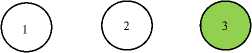

References A Genetic Algorithm Inspired Load Balancing Protocol for Congestion Control in Wireless Sensor Networks using Trust Based Routing Framework (GACCTR)
- C.Y.Wan, S.B.Eisenman and A.T. Campbell, "CODA: Congestion Detection and Avoidance in Sensor Networks", SenSys' 03, Los Angeles, USA, pp. 266-279, ACM, Nov 2003.
- Bret Hull, K. Jamieson, H. Balakrishnan, "Mitigating Congestion in Wireless Sensor Networks", SenSys' 04, Baltimore, Maryland, USA ACM, Nov 2004.
- Y. Sankarasubramaniam, O.Akan, and I.Akyildiz, " Event-to-sink reliable transport in wireless sensor networks", In Proc. Of the 4th ACM Symposium on Mobile Ad Hoc Networking & Computing ( MobiHoc 2002), pages 177- 188. Annapolis, Maryland, June 2003.
- C.Y.Wan, A.T. Campbell, and L. Krishnamurthy, " PSFQ : a reliable transport protocol for wireless sensor networks", In Proc of first ACM International workshop on Wireless Sensor Networks and Applications ( WSNA 2002 ), pages 1-11, Atlanta, September 2002.
- Theodore Zahariadis, Helen C. Leligou, Panagiotis Trakadas and Stamatis Voliotis, "Mobile Networks Trust Management in Wireless Sensor Networks", European Transactions on Telecommunications, 2010; 21:386-395.
- A.Raha, S.S. Babu, M.K. Naskar, "Geometric Mean based Trust Management system for WSNs (GMTMS)", published in WICT 2011 Mumbai, 2011.
- Mohammad Momani, Ph.D thesis on " Bayesian methods for modeling and management of Trust in Wireless Sensor Networks", University of Technology, Sydney, July, 2008.
- S.S. Babu, A. Raha, and M.K.Naskar, "A Direct Trust Dependent Link State Routing Protocol using Route Trusts for Wireless Sensor Networks (DTLSRP)", Wireless Sensor Network journal, USA, pp. 125-134, April 2011.
- A. Raha, M.K.Naskar, S.S. Babu, Omar Alfand and Dieter Hogrefe, "Trust Integrated Link State Routing Protocol for Wireless Sensor Network (TILSRP), published in Proc. Of 5th IEEE ANTS 2011, Dec 2011.
- Mani Zarei, Amir Msoud Rahmani, Avesta Sasan, Mohammad Teshnehlab, "Fuzzy based trust estimation for congestion control in wireless sensor networks", 2009 International Conference on Intelligent Networking and Collaborative Systems.
- Mani Zarei, Amir Msoud Rahmani, Razieh Farazkish, Sara Zahirnia, "FCCTF: Fairness Congestion Control for a distrustful wireless sensor network using Fuzzy logic", 2010 10th International Conference on Hybrid Intelligent Systems.
- D. Goldberg, B. Karp, Y. Ke, S. Nath, and S. Seshan, "Genetic algorithms in search, optimization, and machine learning", Addison-Wesley, 1989.
- A. Chakraborty, S. K. Mitra and M. K. Naskar, "A Genetic Algorithm inspired Routing Protocol for Wireless Sensor Networks", accepted in the International Journal of Computer Intelligence- Theory and Practice, number 6 vol. 1, 2011.
- G. Nagib and W. G. Ali, "Network Routing Protocol using Genetic Algorithms", published in the International Journal of Electrical & Computer Sciences, IJECS-IJENS, Vol. 10, No. 02.
- Bavitha R and Hemalatha R, "Optimisation of Path using Genetic Algorithm for Wireless Sensor Networks", published in the International Journal of Communications and Engineering, Volume 05 – No.: 05, Issue 03, March 2012.
- Wikipedia, "Fitness proportionate selection", July 2012.
