A heuristic strategy for sub-optimal thick-edged polygonal approximation of 2-D planar shape

Published Online April 2018 in MECS DOI: 10.5815/ijigsp.2018.04.06

Computer vision technology has recently witnessed a very rapid growth with the advancement of computational processing ability leading to widespread demand for automated shape analysis in numerous computer vision applications [2], [36], [37]. Extracting meaningful information and features from the contour of 2-D digital planar curves has been widely used for shape modeling [3], [4]. Detection of dominant points (DP) along the contour to represent visual characteristics of a shape has always been a challenging aspect for effective shape modeling. Dominant points are commonly identified as the points with local maximum curvatures on the contour.

Over the years, many algorithms have been developed to detect dominant points. Most of them can be classified into two categories: (1) Polygonal approximation approaches and (2) Corner detection approach [5]. We shall confine our discussion to polygonal approximation approach. Polygonal approximation of a closed digital curve has always been considered as an important technique to reduce the memory storage and the processing time for subsequent analysis of image objects. An exact method to the polygonal approximation problem is impractical due to the intensive computations involved. However, for many decades researchers have been exploring lot of techniques for effective polygonal approximation as discussed below.

• A.    Related Work

The design of a polygonal approximation algorithm not only impacts on the compression ratio of the data volume but also affects the accuracy of the subsequent image analysis tasks [1]. The most popular polygonal approximation algorithm proposed by Ramer [6] recursively splits a curve into two smaller pieces at a point with maximum deviation from the line segment joining two curve end points and a threshold value for the maximum deviation is preset to terminate the recursive process. N.L. Fernandez-Garcia et al. [7] proposed a modified symmetric version of Ramer’s polygonal approximation scheme by computing normalized significance level of the contour points. Sklansky and Gonzalez [8] proposed a cone-intersection method to sequentially partition a digital curve. Wall and Danielsson [9] developed a threshold-based method for partitioning a curve by finding the point at which the deviance of area per unit length surpasses a stipulated value. Ansari and Delp [10] initially found the points with the greatest curvature by Gaussian Smoothing method and then used a split-and-merge procedure to discover the dominant points. Kankanhalli [11] offered an iterative dominant point extraction solution by initially specifying four dominant points and their support regions. F.J. Madrid-Cuevas et al. [12] adopted an efficient split or merge strategy on analyzing the concavity tree of a contour to obtain polygonal approximation with modest computational complexity.

All of the aforementioned algorithms are mostly aimed to offer rapid solutions to the problem sacrificing the optimality. The detection of an optimally approximated polygon was demonstrated by Dunham [13] with a dynamic programming algorithm. Another method of computing the polygonal description by analysis of coupled edge points followed by grouping them for formation of lines or arcs was given by Rosin and West [14]. Key feature selection using genetic algorithm has always been a popular approach among data scientists for reducing redundancy [15]. Huang and Sun [16] proposed a genetic algorithm-based approach to find the polygonal approximation. Xiao et al. [17] adopted a split-and-merge algorithm for describing curves with robust tolerance. Massod’s approach [18], [19] starts from an initial set of dominant points where the integral square error from a given shape is zero and iteratively deletes most redundant dominant points till required approximation is achieved. Kolesnikov’s [20] framework treats the problem of the polygonal approximation with a minimum number of approximation segments for a given error bound with L2-norm and the solution is based on searching for the shortest path in a feasibility graph that has been constructed on the vertices of the input curve. E.J. Aguilera-Aguilera’s [21], [22] solution relies on Mixed Integer Programming techniques for minimization of distortion to obtain optimal polygonal approximation of a digital planar curve. Optimal algorithms are best in producing polygonal approximation but these are computationally very heavy. Therefore, these are of hardly any practical use except as reference for evaluation of non- optimal results. A near optimal algorithm with improvement in computational efficiency may be the most suitable option in most applications.

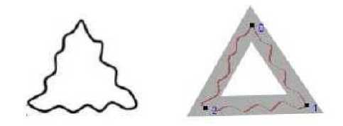
Fig.1. Proposed Scheme: Thick-Edged Polygonal Approximation.

• B.    Objective

Keeping computational efficiency as primary focus, we propose a greedy heuristic based framework for near-optimal detection of dominant boundary-points through an optimally thick-edged polygonal approximation scheme. It is observed that most of the traditional polygonal approximation schemes fail to address the presence of bumpy irregularities along the contour effectively as they sometimes tend to produce misleading polygonal representation either with too many sides or with too few sides. Our proposed framework attempts to handle such noisy curve using a thick-edge polygonal approximation wherein each edge can have reasonably varied thickness. Fig. 1 intuitively demonstrates suitability of the proposed strategy.

The paper is organized as follows. In Section 2, we intro- duce the proposed framework with formulation of the problem from digital geometric perspective. Section 2 illustrates our employed heuristic search algorithm along with its computational complexity. Section 3 details about the experimentation for evaluating the merit of our method and the experimental results are compared with others.

• II.    Proposed Framework

As mentioned earlier the proposed scheme for detecting dominant boundary points is based on polygonal approximation of closed curve. In discrete geometry, the closed contour of an object can be treated as a curve consisting of a sequence of boundary points [23]. Usually, contour extraction in terms of discrete curve by tracing boundary points using Moor’s strategy [1] is a very popular pre-processing technique to work on the shape of a digital image object. Below, we formulate the problem of approximating a discrete curve in terms of optimally thick-line leading to O(n) algorithm for solving it.

• A. Problem Formulation: Fitting Thick Line to a Discrete Curve

A discrete curve consists of a sequence of points in discrete space Z ² , where Z is the set of integers. In this paper, a geo- metric model is used to describe a thick line for approximating a discrete curve by confining the sequence of curve points in discrete space Z ² . A few terminologies are defined below for illustrating the model conveniently with reference to Fig. 2.

Definition 1. A thick line, denoted by L ( a , b , w ) , is a pair of parallel lines defined by l_x : ax + y + b = 0 and l ₂ : ax + y + b = 0 where w specifies the thickness.

Definition 2. A thick line L^D ( a , b , w ) is for a sequence of discrete points D ( L ) termed as valid thick line if it confines D ( L ) by satisfying following condition.

D ( L ) = ( x , y ) e Z ²:0 <  ax + y + b <  w (1)

Definition 3. An optimal thick line L^D ( a , b , w ) for D ( L ) is a valid thick line for which the thickness $w$ is minimum. It can be mathematically expressed as below.

L Dpt ( a , b , w ) = arg min w L D ( a , b , w )         (2)

The pair of parallel lines ( l , l ) defining the thick line L^D ( a , b , w ) for d ( L ) essentially forms support lines of D ( L ) and the distance between the pair corresponds to the thickness. Using the above described model, the thick line fitting problem can be formulated as below.

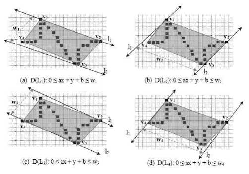
Fig.2. Thick Lines for a Discrete Point Sequence.

Problem: Given a finite sequence of discrete points D, obtain L^D ( a , b , w ) by finding a pair of parallel lines such that

• (1)    The pair forms support lines for D.

• (2)    The distance in between the pair of lines is the smallest possible distance to confine D.

Observation 1. Given a sequence of discrete twodimensional points D and its convex-hull CH ( D ) , there exists a valid thick-line L^D ( a , b , w ) defined by a pair of support lines ( l , l ) such that

• (1)    l is coincident with an edge e_x of CH ( D ) .

• (2)    l is another straight line passing in parallel with l through a vertex v_k  of CH ( D ) which is

farthest from e . The vertex v is termed as antipodal vertex for edge e . The pair ( v , e ) can be termed as antipodal vertex- edge pair and the distance d ( v , e ) gives the measure of the antipodal distance for the pair ( V_k , e ) .

Illustration 1. In Fig. 2, a set of valid thick lines for a sequence of discrete points ( D ( L )) are shown. Every valid thick line is defined by a pair of support       lines        l_v : ax + y + b = 0        and

• l ₂    : ax + y + b = w where w specifies the thickness.

The convex hull for the sequence can also be generated with  the  vertices  {v ,v ,v ,v } to  confine  the sequence. In each figure, one of the support lines of the corresponding thick-line is coincident with one of the edges of the convex hull. For example, in Fig. 2(a) the sequence is confined within the thick line D(L1) defined by      a      pair      of      support      lines

• l _t:    ax + y + b = 0 and    l ₂: ax + y + b = w,   .

Interestingly, l is coincident with e : (v ,v ) and v is antipodal vertex for e as it is farthest from e among all other vertices through which l  passes through. The antipodal distance d(v3, ex) = wx  for the antipodal vertex-edge pair (v3, ex) is the thickness of D(L) ={(x,y) e Z2: 0 < ax + y + b < w,} .

Observation 2. Given a sequence of discrete two dimensional points D and its convex-hull CH (D) , determining an optimal thick-line LD (a, b, w) for D(L) is equivalent of finding an antipodal vertex-edge pair (v, e)    for which the antipodal distance is minimum. The observation can be expressed mathematically as below considering all possible antipodal vertex-edge pair of convex-hull CH (D) .

• ^{( v} ,    ^e ) opt = arg min d ( v , e ) ^{( V , e i )}         ⁽³⁾

Illustration 2. In Fig. 2, as illustrated above a set of valid thick lines with different thickness confines a sequence of discrete 8-connected points D ( L ) . Every thick line corresponds to an antipodal vertex-edge pair of the confining CH ( D ). With close observation, it is found that the distance d ( V ₃, e_x ) = w_x for the antipodal vertex-edge pair ( v , e ) is minimum among all four-antipodal vertex-edge pairs. This observation leads to the conclusion that the optimal thick line L^D ( a , b , w ) for D ( L ) corresponds to the antipodal vertex-edge pair ( v , e ) .

Observation 2 . Given a convex-hull CH ( D ) with a clockwise sequence of vertices: { v , v ,..., v } and three consecutive vertices v , v , and v , the following propositions are true if vertex v forms an antipodal vertex of the edge e : ( v , v ) .

• (1)    V_k is farthest from e_i+1 among the clockwise sequence of vertices { v , v ,..., v } . i t implies

that the antipodal vertex for the edge e must be a vertex belonging to the clockwise sequence e { V_k , V_{k p}..., V } with v_k being first candidate under consideration.

• (2)    If d ( V k , e i + 1 ) >  d ( V k _{+ 1}, e_{i + 1}) then V k  is also an

antipodal vertex for the edge e otherwise v can be checked against v as a new candidate for the antipodal vertex to the edge e . The comparison of v against v can be done in similar manner with which previous candidate v is compared against v .

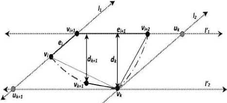
Fig.3. Observation 3.

Proof. The proof is provided with reference to Fig. 3 which corresponds to the given convex hull with vertices being marked in clockwise order as stated in observation 3. In Fig. 3, a pair of parallel lines namely l and l act as support lines for the convex hull such that l is coincident with e and l passes through the vertex v . There are another pair of parallel lines l and l wherein l is coincident with e and l passes through the vertex v . Under such circumstance, the following observations are evident in order to satisfy the convexity property of a convex hull.

• (1)    Since v is farthest vertex from e , any vertex

Vj e { v _/+2, v _/+3,..., v_k } must lie to the left side of l (i.e. on the side where l lies).

• (2)    Since every vertex Vj e { v_{/+ 2}, V _/+3,..., V_k } forms a convex vertex, v must also lie to the right side of the line segment joining vertices v and v ⁽i.e. ^V k ^Vi + 2 ).

These two criteria lead to the fact that any arbitrary vertex Vj e{V/+2, V/+3,..., Vk} must lie in the triangular region AVkVi+\Uk (Fig. 3). The distance of any point lying in AVkVi+1Uk from e 3 is always less than dk (i.e. the distance of v from e ). Therefore v is farthest from e among the clockwise sequence of vertices{V+2,V^,...,Vk} .

Algorithm 1: Find Optimal Thick Line for dis crete CURVE

10 II

Input: Global PointList: A list of points representing the discrete curve

Output: Global ThickLine_Opt :< e,, Vk >* It corresponds to annpodai-pair(edge(Vi, Vi^-i), Vk) with minimum antipodal distance.

Generate convex-hull with clockwise vertex sequence:(vi, «2,—»vn) from the giren list of curve-points

Vk t~~ Farthest vertex foredgp(v„, vi) found on linearly traversing the list of vertices {vi, va^v»}

5™„ <- dist(edge(u„, ui),u_t)

il-2

while i < n do

6k 4— dist^cdge^Ut-l , v,), Vfc)

5t+i -f-distCet^efui-i,^),^!)

if Sk < ^₊1 Iheo

| jfc-e—Jfc + 1

end else if 5k < 5min then

Smin <- 5k

ThickLine_Opt -t— ThickLina :< e«—i, Vk >  for antipodal-pair(edge(Vi—i, Vi),Vk)

end i -4— i-hl end end return ThickLineOpt

Let dk = d (Vk, ei+1)and dk+1 = d (Vk+1, ei+1)  . If dk > dk+x then Vt j must lie in the triangular region AV u V (Fig. 3) to satisfy the property of convexity. Any point lying inside AV^U-^V cannot be as far as Vk from e . Therefore v can be treated as the antipodal vertex ofe .

Based on the previous observation, we now present an algorithm (Algorithm 1: fitThickLine) below to find an optimal- valid-thick line for a discrete curve. Given a discrete curve of n points, the time complexity of the algorithm is O ( n log n ) if we follow graham-scan strategy for convex-hull generation.

• B. Thick-Poly-line Approximation of Contour

In discrete geometry, a poly-line is a connected series of line segments. The poly-line is extensively used for approximating a discrete curve with a polygon in order to represent its shape [24]. A poly-line is formally specified by a sequence of points called its vertices. There are many computer vision- b a s e d applications based on shape analysis framework wherein a digital curve representing   various   complex   contours   need simplification. A digital curve can be effectively simplified by poly-line without loss of its inherent visual property. Techniques for poly-line approximation of digital curve have been driving interest among the researchers for decades. The idea of poly-line approximation based on digital geometry has recently been explored extensively for simplified modeling of a shape [24], [23]. In this paper, we have focused on developing an approximation strategy to determine polygonal representation of a shape using special thick-poly-line wherein every line segment is an optimal thick line corresponding to its respective curve segment.

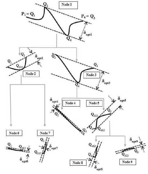
Fig.4. Greedy Best-First Spitting Strategy.

Cost of Fitting Optimal-Thick-line: Given a discrete curve segment with end points P and P , its confining optimal thick line ThickLine ( P , P ) as illustrated before also associates a cost in terms of its thickness. Cost associated with fitting a Curve ( P , P ) using ThickLine ( P , P ) :

Cost(P,P ) = Thickness(P, P ) (4)

Splitting Scheme: A curve is split into two segments at one of its convex-hull-vertices Q and the vertex at which the curve is split is termed as PivotVertex in our scheme. Every convex-hull-vertex Q except the curve end points can split the curve into two proper segments but only one vertex would be chosen as PivotVertex depending on an optimal criterion as expressed through following equations. SplitCost(P, P ,Q ) denotes the heuristic cost associated for choosing Q as PivotVertex and it is computed based on thick-line-fitting-costs of the sub-segments generated on splitting the Curve(P, P ) at Q . The objective criteria of selecting PivotVertex is to minimize aggregate costs of two split-segments as well as difference between their individual costs. SplitCost(P, P ,Q) considers both aggregate-cost and cost-difference of two split-segments as expressed below. In Figure. 4 at root level QQ Q Q represents vertices of the convex hull of a Curve(P, P ) and as per our scheme, the curve can be split at two convex-hullvertices namely Q or Q but Q is selected as PivotVertex because SplitCost(P, P ,Q ) is less thanSplitCost(P, P ,Q ) . The splitting scheme under repetitive application based on greedy Best-First-Heuristic [25] exploration leads to the generation of a tree-like decomposition flow-structure as presented in Figure. 4.

CostSum ( P , P n , Q i ) = Cost ( P , , Q i ) + Cost ( Q i , P n )

CostDiff ( P , P n , Q i ) = ABS ( Cost ( P , Q i ) - Cost ( Q i , P n )) SplitCost ( P , , P n , Q i ) = CostSum ( P , P n , Q i ) + CostDiff ( P , , P n , Q i ) PivotVertex = arg min^ SplitCost ( P , P_M , Q_ )

Greedy   Best-First-Heuristic   Based Exploration

Strategy: Greedy Best-First-Heuristic process explores a search-tree by expanding the most promising node chosen according to heuristic cost [25]. The above illustrated splitting scheme under greedy Best-First-Heuristic based exploration generates a tree-like decomposition flow-structure as presented in Figure 4. Each node of the decomposition tree represents a curve segment and undergoes further splitting operation if the termination condition is not met. The termination of the repetitive splitting operation takes place whenever number of leaves representing yet-to-be decomposed curve segments in the recursion tree reaches the user-specified intended number of dominant points. Under such exploratory repetitive splitting strategy, at every step until termination, we are to select a tree-node representing a curve segment which is split on the next move. The selection is performed based on greedy best-first-heuristic [25] strategy which considers most promising node with minimum SplitCost ( P , P , Q ) for subsequent exploration. The proposed best-first-heuristic strategy examines tree-nodes which are not yet decomposed and selects a node from them whose heuristic cost is minimum among all yet-to-be decomposed nodes irrespective of tree-levels. At every splitting step, two more child-curves are generated leading to generation of two new curve segments as candidates       for       subsequent      exploration.

C. Proposed Algorithm

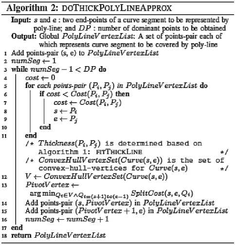
The greedy best-first-heuristic algorithm (Algorithm 2:   doThickPolyLineApprox)   developed   for approximating a closed digital curve with thick-poly-line is formally presented in this section. The digital curve is stored as an ordered list of two-dimensional points. Our proposed algorithm repetitively splits the curve leading to generation of a tree like exploration as described earlier wherein each tree-node represents a curve segment. At every exploratory step, the best-first-strategy of the proposed method selects the most suitable node which is yet to be split and subsequently the splitting scheme of the proposed framework splits the curve segment corresponding to the selected node into two smaller segments. The repetitive splitting operation terminates whenever number of leaves i.e. yet-to-be decomposed curve segments in the recursion tree reaches the user-specified desired number of dominant segments.

Illustration of the Proposed Algorithm 2. Figure 4 represents a tree-like decomposition flow-structure rendered while tracing our proposed algorithm (doThickPolyLineApprox) to fit a given curve with five poly-lines generating ten dominant points. Our proposed strategy splits the original curve at node- 1 into two curve segments at node-2 and node-3 respectively based on previously described splitting-scheme. Since, the cost of the curve at node-3 is found to be larger than that of node-1, the curve at node-3 is selected next for further decomposition. The sequential order in which the nodes in Figure 4 would be selected for successive decomposition depends on greedy best-first-heuristic strategy [25]. For a given curve as shown in Figure 4, the exploration of our proposed algorithm would select candidate nodes in a specific sequential order driven by the greedy best-first-heuristic strategy. For the stated example, node-1 is selected first and then node-3 is chosen as next decomposition candidate followed by selection of node-5, and lastly node-2 gets selected to undergo splitting operation. Ultimately on termination, the proposed scheme produces five curve segments at node-4, node-6, node-7, node-8 and node- 9 respectively as leaves of the decomposition tree, thereby generating ten dominant points.

Average Time Complexity:    The average time complexity of the algorithm for a curve of N points is given by the recurrence relation 6. At every exploratory step, the proposed thick-line fitting algorithm involves generation of a convex hull and determination of optimal-valid-pair for finding optimal thick-line. Convex-hull generation takes O (N log N) time complexity as we have used Graham-Scan [1] method while the determination of optimal-valid-pair requires O(N) time complexity. Considering both, the proposed thick-line fitting algorithm effectively causes O (N log N) time complexity. Additionally, at each step, the curve splitting heuristic scheme of the proposed framework explores the vertices of convex-hull of the given curve as spitting candidate pivot points which also involves the same time complexity as required for convex-hull generation. The average time complexity of the overall algorithm can be proved to be approaching O (N log N) .

{ |       N - 1

N log N +-----x £ { T ( i ) + T ( N - i + 1 ) },    N >  2.

N - 2     . . 2

0,                                                        otherwise.

• III.    Experimental Results And Analysis

Evaluation of performance is a crucial problem for such frameworks, mainly due to the subjectivity of the human vision-based judgment. The performance of such frameworks has commonly been evaluated by conducting experiments on the Teh Chin Curves [26] and some figures of mpeg- 7 database [27]. The merit of such a scheme depends on how closely a polygon comprising small but significantly important dominant points can represent the contour. It is intuitive that the best way to compare results qualitatively can only be performed by visual observation which fails to assess the relative merits of the various algorithms precisely. Therefore, quantitative approach is inevitable for automated measuring performance of such frameworks. The most widely used criteria, for estimating effectiveness of the scheme considers–a) Amount of data reduction and b) Closeness to the original curve . Generally, amount of data reduction is measured as the Compression Ratio ( CR ) and the closeness to the original shape is popularly measured in terms of Integrated Square Error ( ISE ) or Average Max Error ( AvgMaxErr ) [28]. These values are obtained using following expressions where n is the number of contour points and n d is the number of Dominant Points (DP).

n

ISE = V {error x error } i=1

MaxErr = max{ error }

1 < i <  n           i

1 n d - 1

AvgMaxErr =---V {MaxErr } nd-i i=1

CR = —, FOM = — n         ISE

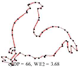
Table 1. Result: thick-edge polygonal approximation: a) bell-10, b) device6-9, c) chicken-5

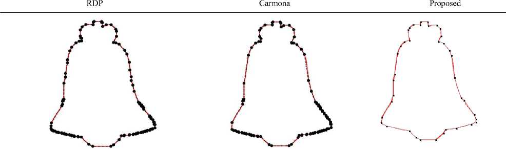
a) DP = 110, W E2 = 1.52                   a) DP = 104, W E2 = 3.96

a) DP = 36, W E2 = 0.72

There must be a tradeoff between the two parameters since high compression ratio leads to high ISE whereas sustaining low ISE may lead to lower compression ratio. This means that comparing algorithms based on only one measure is not sufficient. In order to justify this trade off, Sarkar [29] combined these two measures as a ratio, producing a normalized figure of merit (FOM) which can be computed as ration of CR and ISE. Unfortunately, the FOM as proposed by Sarkar turns out unfit for comparing approximations with different number of points [30] and a parameterized version of weighted sum of squared error ( we = ISE ) has n CRk been proposed in [31]. Carmona [32], [33] showed that the value k = 2 leads to the best performance.

In summary, when the number of DPs is same, FOM can be considered as the most sensible quantitative parameters for comparison of polygonal approximation results [19]. However, in case of different number of DPs, we have relied on Carmona’s [33] observation considering weighted sum of squared error (WE 2 ) as evaluating measure to draw comparative observations.

These comparative observations are presented in Table 1 along with figures. Comparative results with same number of DPs are carried out on popular Teh- Chin curves. The outcomes of our proposed algorithm with various possibilities of dominant points are presented in Table 2 to demonstrate qualitative differences depending on varying number of DPs. Table 3 lists the results of proposed algorithm in comparison with some commonly referred algorithms [18] on the basis of FOM while keeping compression ratio (CR) identical with respective comparative algorithms. In overall assessment, the performance of the proposed algorithm is reasonably good as compared to others. In addition to the quantitative parameters as discussed above there are also few other factors which must also be explored while evaluating any polygonal approximation algorithm. These are discussed below.

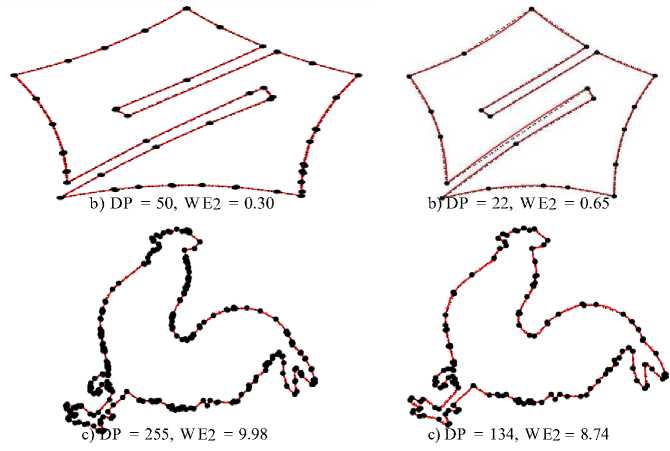
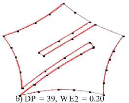
Table 2. Result: thick-edge polygonal approximation: a) chromosome, b) semicircle, c) leaf

D P = 10

DP = 20

DP = 30

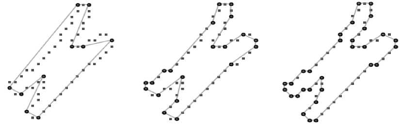
a) AvgMaxErr = 0.58

a) AvgMaxErr = 0.22

a) AvgMaxErr = 0.06

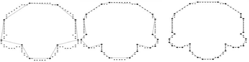
b) AvgMaxErr = 1.65

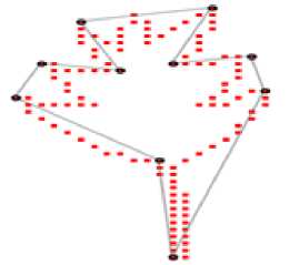
c) AvgMaxErr = 2.12

b) AvgM axErr = 0.47

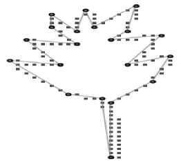
c) AvgMaxErr = 0.47

b) AvgMaxErr = 0.19

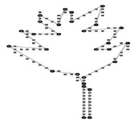
c) AvgMaxErr = 0.26

Table 3. Comparative results

Shape	Method	CR	FOM
Chromosome	Ray and Ray [34]	3.33	0.59
(n = 60)
	Proposed	3.33	0.82
	Wu [5]	3.53	0.70
	Proposed	3.53	0.80
	Teh and Chin [26]	4.00	0.55
	Proposed	4.00	0.75
Semicircle	Ray and Ray [34]	3.52	0.29
(n = 102)
	Proposed	3.52	1.01
	Ansari and Huang [35]	3.64	0.20
	Proposed	3.64	0.86
	Wu [5]	3.78	0.41
	Proposed	3.78	0.86
	Teh and Chin [26]	4.64	0.22
	Proposed	4.64	0.42
Leaf	Ray and Ray [34]	3.75	0.25
(n = 120)
	Proposed	3.75	0.40
	Teh and Chin [26]	4.14	0.27
	Proposed	4.14	0.38
	Wu [5]	5.22	0.25
	Proposed	5.22	0.29

Table 4. Result: effect of thickness on no. Of dps

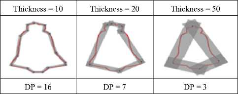
Consistency: Consistency guarantees that if the number of DPs is plotted against the error measure, the error value should monotonically decrease with the increase in number of DPs. Most of the algorithms are found to be non- monotonic [30] which can pose a problem for a user as it is difficult to select an appropriate parameter if the effect of change in value is not predictable. Fig. 5 shows how thickness governs number of DPs and Fig. 6 shows the influence of number of DPs on error-measure in the proposed scheme.

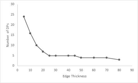
Fig.5. Thickness vs Number of DPs, Shape: bell-10.

Flexibility : A flexible algorithm for polygonal approximation should be able to determine polygonal approximation for any reasonable number of DPs. Proposed algorithm can meet such flexible requirements. Generally, flexibility in an algorithm is introduced by certain parameters. In the proposed framework, thickness of the approximating polygon-side can also be specified by the user instead of specifying number of DPs to be produced and such a scheme automatically deter- mines possible number of DPs with user specified thickness of approximating polygonal side. The effect of thickness on the number of DPs is shown in Fig. 5 and in Table 4. It is clear that with the increase of thickness, lesser number of DPs is produced in the approximation.

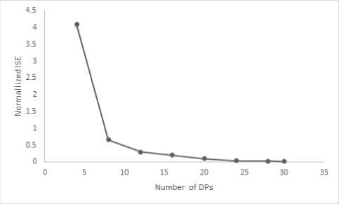
Fig.6. Number of DPs vs ISE, Shape: semicircle.

Computational Efficiency: Optimal algorithms are best in producing polygonal approximation but these are computationally very heavy. Therefore, these are of hardly any practical use except acting as reference for evaluation of non-optimal results. A greedy algorithm with improvement in approximation accuracy may be the most suitable option in most applications. Results of the proposed greedy algorithm can be rated as close to acceptable accuracy with computational time reasonable enough for any standard shape. Fig. 7 presents a graph showing computational time plotted against number of DPs along with the impact of boundary length on computational time. It has been observed experimentally as evident in Fig. 7 that the execution time grows at moderate rate with the increase of shape contour length.

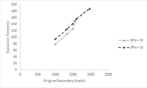
Fig.7. Graph: Execution Time vs Shape Boundary Size (n).

• IV.    Conclusion

This paper presents a new idea for dominant point detection on an object’s contour using a special thickedge polygonal approximation framework. Experimental results have shown that the proposed algorithm can generate efficient and effective polygonal approximations for digital planar curves. The new proposal explores a unique idea of piece-wise thick-line-fitting to a curve based on digital geometry and uses greedy best-first heuristic strategy to repetitively split a curve for generating dominant points. The proposed algorithm attempts to obtain fairly accurate solution with average computational         complexity         approaching asymptotically O (N log N) for large curve. The desired number of vertices of a shape-approximating polygon is ideally assumed to be as few as possible without losing dominant visual characteristics of the shape. As per our observation, the proposed framework especially   seems   to   perform   fairly well in approximating the shape when the number of dominant points is close to actual number of contourkey points. In our proposed work, the requisite of a larger edge-thickness leads to the generation of a shapeapproximating polygon having fewer vertices in terms of dominant points. In overall assessment, the proposed framework successfully attempts to incorporate robustness against noisy contours of standard shapes with automated tuning of thickness of the edges of shape approximating polygon.