A Hierarchical Load Balancing Policy for Grid Computing Environment

Recent researches on computing architectures led the computing environment to be mapped from the traditionally distributed systems and clusters to the Grid environments. Computing Grid is hardware and software infrastructure that provides dependable, consistent, pervasive, and inexpensive access to high-end computational capabilities. It enables coordinated resource sharing within dynamic organizations consisting of individuals, institutions, and resources, for solving computationally intensive applications. Such applications include, but not limited to meteorological simulations, data intensive applications, research of DNA sequences, and nanomaterials. It supports the sharing and coordinated use of resources, independently of their physical type and location, in dynamic virtual organizations that share the same goal. Thus computing grid is designed so that users won't have to worry about where computations are being performed [1-4].

Basically, grid resources are geographically distributed computers or clusters (sites), which are logically aggregated to serve as a unified computing resource. The primary motivation of grid computing system is to provide users and applications with pervasive and seamless access to vast high performance computing resources by creating an illusion of a single system image [1,3,5-7]. Grid Computing is becoming a generic platform for high performance and distributed computing due to the variety of services it offers such as computation services, application services, data services, information services, and knowledge services. These services are provided by the servers or processing elements in the grid computing system. The servers and the processing elements are typically heterogeneous in the sense that they have different processor speeds, memory capacities, and I/O bandwidths [5,8].

Due to uneven task arrival patterns and unequal computing capacities and capabilities, the computers in one grid site may be heavily loaded while others in a different grid site may be lightly loaded or even idle. It is therefore desirable to transfer some tasks from the heavily loaded computers to the idle or lightly loaded ones in the grid environment aiming to efficiently utilize the grid resources and minimize the overall mean task response time. The process of load redistribution is known as load balancing [2,5,7-10].

In general, load balancing policies can be classified into static or dynamic [10,11]. In static load balancing policies, the load balancing decisions are made deterministically or probabilistically at compile time and remain constant during runtime. They are not affected by the runtime system state. In contrast, dynamic load balancing policies attempt to use the runtime system state information to make more informative load balancing decision. In [10,11], the authors present classification schemes for dynamic load balancing policies which differ in number and type of parameters. Dynamic load balancing policies in turn can be classified into centralized or decentralized (distributed) in terms of the location where the load balancing decisions are made.

In centralized load balancing policies, the parameters necessary for making the load balancing decision are collected at, and used by, a single resource (decision maker) i.e. only one resource acts as the central controller and all the remaining resources act as slaves. Arriving tasks to the system are sent to controller, which distributes tasks on the slaves aiming to minimize the overall system mean task response time. The centralized policies are more beneficial when the communication cost is less significant, e.g. in the shared-memory multiprocessor environment. Many authors argue that this approach is not scalable, because when the system size increases, the load balancing decision maker may become the bottleneck of the system and the single point of failure [9, 10].

On the other hand, in the decentralized load balancing policies, all computers (nodes) in the distributed system are involved in making the load balancing decision. Since the load balancing decisions are distributed, many researchers believe that the decentralized load balancing policies are more scalable and have better fault tolerance. But at the same time, it is very costly from the communication time point of view to let every computer in the system obtains the global system state information. Hence, in the decentralized mechanisms, usually, each computer accepts the local task arrivals and makes decisions to send them to other computers on the basis of its own partial or global information on the system load distribution [3,9,10,11]. It appears that this policy is closely related to the individually optimal policy, in that each job (or its user) optimizes its own expected mean response time independently of the others [9,10].

Although the load balancing problem in traditional distributed systems has been intensively studied [9,10], the load balancing algorithms for traditional distributed environments do not work directly in grid environments, because grids have a lot of specific characteristics, like heterogeneity, autonomy, scalability, adaptability and resources computation-data separation, which make the load balancing problem more difficult. Therefore, in the grid environment it is essential to consider the impact of various dynamic characteristics on the design and analysis of scheduling and load balancing policies [1214].

In this paper, we propose a fully decentralized two-level load balancing policy for the grid computing environment. The proposed load balancing policy takes into account the heterogeneity of the grid computational resources. It distributes the workload based on the resources occupation ratio and the communication cost. As in [15], we focus on the steady-state mode, where the number of tasks submitted to the grid is sufficiently large and the arrival rate of tasks does not exceed the grid overall processing capacity. The class of problems addressed by the proposed load balancing policy is the computation-intensive and totally independent tasks with no communication between them. An analytical model based on queuing theory is presented. A simulation model is built to evaluate the performance of the proposed load balancing policy.

The rest of this paper is organized as follows: Section II presents related work. Section III describes the grid model and assumptions. Section IV introduces the proposed grid load balancing policy. Section V presents an analytical queuing model for a local grid manager. In section VI, the simulation environment and results are discussed. Finally, Section VII summarizes this paper.

• II.    Related works and motivations

Recently, many papers have been published to address the problem of load balancing in Grid computing environments. Some of the proposed grid computing load balancing policies are modifications or extensions to the traditional distributed systems load balancing policies. In [16], a brief survey of job scheduling and resource management in grid computing is presented. The authors of [17] and [18] presented a static load balancing policy in a system with servers and computers where servers balance load among all computers in a round robin fashion. It requires each server to have information on status of all computers as well as the load allocated by all other servers. In [19] the authors presented a load balancing policies for the computational grid environment in which the grid scheduler selects computational resources based on the task requirements, task characteristics and information provided by the resources. Their performance metrics was to minimize the Total Time to Release (TTR) for the individual task. TTR includes processing time of the task, waiting time in the queue, transfer of input and output data to and from the resource. The load balancing policies in [20] introduce a task migration mechanism to balance the workload when any of the processing elements become overloaded but they does not consider the resource and network heterogeneity. In [21], the authors proposed a ring topology for the Grid managers which are responsible for managing a dynamic pool of processing elements. The load balancing algorithm was based on the real computers workload which is not applicable because of its huge overhead cost. Many hierarchical load balancing policies in grid computing are referred in [1,8,12,21-24] where load balancing policies are implemented at various levels of grid resources to reduce mean response time of the grid application.

In [22], the authors presented four strategies for resource allocations in a 2-level hierarchy grid computing model. They studied the performance of these strategies at the global scheduler and local scheduler levels. Also, in [1,12] the authors presented tree-based models to represent any Grid architecture into a tree structure. The model takes into account the heterogeneity of resources and it is completely independent of any physical Grid architecture. However, the policies presented in [1,22] did not provide any task allocation procedure and they did not consider the communication cost between clusters. Their resource management policy is based on a periodic collection of resource information by a central entity (Grid Manager or Global Scheduler), which might be communication consuming and also a bottleneck for the system. In [8] the author presented a two-level load balancing policy that takes into account the heterogeneity of the grid computational resources. It distributes the system workload based on the resources processing capacity which leads to minimize the overall mean task response time and maximize the grid utilization and throughput at the steady state. The model presented in [8] overcomes the bottleneck of the models presented in [1,12,22] by removing the Grid Manager node which centralizes the global load information of all the grid resources but it also doesn't consider the communication cost between clusters as in [1,22]. The same authors of [21] proposed in [23] a hierarchical structure for grid managers rather than ring topology to improve scalability of the grid computing system. They also presented a task allocation policy which automatically regulates the task flow rate directed to a given grid manager.

In this paper, we propose a fully decentralized two-level load balancing policy for computationally intensive tasks on a heterogeneous multi-cluster grid environment. The load balancing decisions in this policy are taken at the local grid manager and at the site manager levels. The proposed policy allows to any site manager to receive two kinds of tasks namely, remote tasks arriving from its associated local grid manager, and local tasks submitted directly to the site manager by the local users in its domain, which makes this policy closer to reality and distinguishes it from any other similar policy. It distributes the grid workload based on the resources occupation ratio and the communication cost. As in [8], the model presented in this paper overcomes the bottleneck of the hierarchal models presented in [1,12,22] by removing the Grid Manager node which centralizes the global load information of all the grid. In contrast to [8], it considers the communication cost between different sites or clusters. The grid overall mean task response time is considered as the main performance metric that need to be minimized. The proposed policy aims to reduce the grid overall mean task response time and minimize the communication overhead. It provides the following unique characteristics of practical Grid computing environment:

Large-scale: As a grid can encompass a large number of high performance computing resources that are located across different domains and continents, it is difficult for centralized model to address communication overhead and administration of remote workstations.

Heterogeneous grid resources: The Grid resources are heterogeneous in nature, they may have different hardware architectures, operating systems, computing power, resource capacity, and network bandwidth between them.

Effects from considerable transfer delay: The communication overhead involved in capturing load information of local grid managers before making a dispatching decision can be a major issue negating the advantages of task migration. We should not ignore the considerable dynamic transfer delay in disseminating load updates on the Internet.

Tasks are non-preemptable: Their execution on a grid resource can't be suspended until completion.

Tasks are independent: There is no communication between tasks.

• III.    System Model

We consider a computing grid model which is based on a hierarchical geographical decomposition structure. It consists of a set of clusters or sites present in different administrative domains. For every local domain, there is a Local Grid Manager (LGM) which controls and manages a local set of sites (clusters). Every site owns a set of processing elements (PEs) and a Site Manager (SM) which controls and manages the PEs in that site. Resources within the site are interconnected together by a Local Area Network (LAN). The LGMs communicate with the sites in their local domains via the corresponding SMs using a High-Speed network. LGMs all over the world are connected to the global network or WAN by switches.

Grid users can submit their tasks for remote processing (remote tasks) through the available websites browsers using the Grid Computing Service (GCS) to the LGMs. This makes the job submission process easy and accessible to any number of clients. The Global Scheduler (GS) at the LGMs distributes the arriving tasks to the SMs according to a load balancing policy which is based on the available information about the SMs. Also, any local site or cluster user can submit his computing tasks (local tasks) directly to the SM in his domain. Hence, any SM will have two kinds of arriving tasks namely, remote tasks arriving from its associated LGM and local tasks submitted directly to the SM by the local users. We assume that local tasks must be executed at the site in which they have been submitted (i.e., they are not transferred to any other site). The Local Scheduler at the SM in turn distributes the arriving tasks on the PEs in its pool according to a load balancing policy which is based on the PE's load information. When the execution of the tasks is finished, the GCS notify the users by the results of their tasks.

A top-down three level view of the considered computing grid model is shown in Fig. 1. It can be explained as follows:

• • Level 0: Local Grid Manager (LGM)

Every node in this level, called Local Grid Manager (LGM), is associated with a set of SMs. It realizes the following functions:

• (i)    It manages a pool of Site Managers (SMs) in its geographical area (domain).

• (ii)    It collects information about its corresponding SMs.

• (iii)    New SMs can join the GCS by sending a join request to register themselves at the nearest parent LGM.

• (iv)    LGMs are also involved in the task allocation and load balancing process not only in their local domains but also in the whole grid.

• (v)    It is responsible for balancing the accepted

workload between its SMs by using the GS.

• (vi)    It sends the load balancing decisions to the

nodes in the level 1 (SMs).

• • Level 1: Site Manager (SM)

Every node in this level, called Site Manager (SM), is associated with a grid site (cluster). It is responsible for:

• (i)    Managing a pool of processing elements (computers or processors) which is dynamically configured (i.e., processing elements may join or leave the pool at any time).

• (ii)    Registering a new joining computing element to the site.

• (iii)    Collecting information such as CPU speed, Memory size, available software and other hardware specifications about active processing

elements in its pool and forwarding it to its associated LGM.

• (iv)    Allocating the incoming tasks to any processing element in its pool according to a specified load balancing algorithm.

• • Level 2: Processing Elements (PE)

At this level, we find the worker nodes (processing elements) of the grid linked to their SMs. Any private or public PC or workstation can join the grid system by registering within the nearest parent SM and offer its computing resources to be used by the grid users. When a computing element joins the grid, it starts the GCS system which will report to the SM some information about its resources such as CPU speed, memory size, available software and other hardware specifications.

Every PE is responsible for:

• (i)    Maintaining its workload information.

• (ii)    Sending instantaneously its workload information to its SM upon any change.

• (iii)    Executing its load share decided by the associated SM based on a specified load balancing

  Communication Network

  

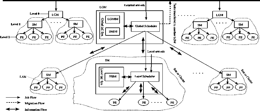
  Figure 1 . Grid Computing Model Architecture

  
  

As it could be seen from this decomposition, adding or removing SMs or PEs becomes very easy, flexible and serves both the openness and the scalability of proposed grid computing model. Also, the proposed model is a completely distributed model. It overcomes the bottleneck of the hierarchal models presented in [1,12,22] by removing the Grid Manager or Global node which centralizes the global load information of all the grid. The Grid manager node can be a bottleneck and therefore a point of failure in their models. The proposed model aims to reduce the overall mean response time of tasks and to minimize the communication costs.

Any LGM acts as a web server for the grid model. Clients (users) submit their computing tasks to the associated LGM using the web browser. Upon a remote task arrival, according to the available load information, the LGM accepts the incoming task for proceeding at any of its sites or immediately forwards it to the fastest available LGM. The accepted rate of tasks will be passed to the appropriate SM based on the proposed load balancing policy. The SM in turn distributes these computing tasks according to the available PEs load information to the fastest available processing element for execution.

• A. System parameters

For each resource participating in the grid the following parameters are defined which will be used later on the load balancing operation.

• 1.    Task parameters: Every Task is represented by a task Id, number of task instructions NTI, and a task size in bytes TS.

• 2.    PEs parameters: CPU speed, available memory, workload index which can be calculated using the total number of jobs queued on a given PE and its speed.

• 3.    Processing Element Capacity (PEC): Number of tasks per second a PE can process. It can be calculated using the CPU speed and an average number of instructions per task.

• 4.    Total Site Manager Processing Capacity (TSMPC): Number of tasks per second the site can process. It can be calculated as the sum of the PECs of all the processing elements of that site.

• 5.    Total Local Grid Manager Processing Capacity (LGMPC): Number of tasks that can be executed under the responsibility of the LGM per second. The LGMPC can be calculated by summing all the TSMPCs for all the sites managed by the LGM.

• 6.    Total Grid Processing Capacity (TGPC): Number of tasks executed by the whole grid per second. The TGPC can be calculated by summing all the LGMPCs for all the LGMs in the grid.

• 7.    Network Parameter: Bandwidth size

• 8.    Performance Parameters: The overall mean task response time is used as the performance parameter.

• IV. Proposed Load Balancing policy

A two-level load balancing policy for the multi-cluster grid computing environment, where clusters are located in different local area networks, is proposed. This policy takes into account the heterogeneity of the computational resources. It distributes the system workload based on the fastest available processing elements load balancing policy. We assume that the tasks submitted to the grid system are totally independent tasks with no inter-process communication between them, and that they are computation intensive tasks. The FCFS scheduling policy is applied for tasks waiting in queues, both at Global scheduler and Local scheduler. FCFS ensures certain kind of fairness, does not require an advance information about the task execution time, do not require much computational effort, and is easy to implement. Since the SMs and their PEs resources in a site are connected using a LAN (very fast), only the communication cost between the LGMs and the SMs is considered.

The proposed load balancing policy is explained at each level of the grid architecture as follows:

• A. Local Grid Manager Load Balancing Level

A LGM is responsible of managing a group of SMs as well as exchanging its load information with the other LGMs. It has Global Information System (GIS) which consists of two information modules: Local Grid Managers Information Module (LGMIM) and the Sites Managers Information Module (SMIM). The LGMIM contains all the needed information about the other LGMs such as load information and communication bandwidth size. The LGMIM is updated periodically by the LGMs. Similarly, the SMIM has all the information about the local SMs managed by that LGM such as load information, memory size, communication bandwidth, available software and hardware specifications. Also, the SMIM is periodically updated by the SMs managed by that LGM. Since the LGMs communicate using the global network or the WAN (slow internet links) while the LGM communicates with its SMs using a High Speed network (fast communication links), the periodical interval for updating LGMIM tG is set to be greater than the periodical interval for updating the SMIM (tS i.e., tG > tS) to minimize the communication overhead. The GS uses the information available in these two modules in taking the load balancing decisions.

When an external (remote) task arrives at ith LGM, its GS does the following steps:

Step 1: Workload Estimation

• (i)    To minimize the communication overhead, based on the information available at its SMIM which is more frequently updated than the LGMIM (since T G >T S ), the GS accepts the task for local processing at the current LGM i if that LGM is in the steady state (i.e., p <1) and goto step 2 else

begin {else}

• a.    Check the task size S in MB.

• b.    Based on the information available at the LGMIM, for every LGM K , K≠i compute the following:

Ck = Rk +---------- ^S ----------,

^{K K}  LinkSpeed ( LGM_i , LGM_k )

K=(1,2,…,i-1,i+1,…,L)

where:

N

• •    R K =---- is the occupation ratio at the

P k

LGM K ; where N is the total number of tasks at the LGM K , and p_K is the total processing capacity of the LGM K .

• •    LinkSpeed(LGM i , LGM k ) is the speed (in Mbps) of communication link between the current LGM i , and the other LGM K , K≠i.

• •    L is the number of LGMs in the whole grid.

• c.    Detecting the fastest available LGM to send the task to it

• (i)    Find the LGM K , K=1,2,…,i-1,i+1,…,L

having the lowest value of C .

• (ii)    Forward the task immediately to the LGM K , update the LGMIM at the GIS and goto step 1 for servicing a new task. end {else}

Note: We assume that a transferred task from LGM i to LGM K for remote processing receives its service at the LGM K and is not transferred to other LGMs (i.e., each task is forwarded at most once to minimize the communication cost).

Step 2: Distributing the workload accepted for processing at the LGM i on its SMs.

• (i)    Based on the information available on the SMIM, for every SM number j managed by the LGM i , compute the following:

с» = R + ---------- , j=( 1 , 2 ,?m )

^{ij ij} LinkSpeed ( LGM_i , SM_j ) where:

• •    S is the task size in MB.

Nij

• •   R ₌ —— is the occupation ratio at the j™ SM

Ptj managed by the LGMi; where Nij is the total number of tasks at the jth SM managed by the LGMi, and pj is the total processing capacity of jth SM managed by the LGMi.

• •   LinkSpeed(LGM i , SM j ) is the speed (in

Mbps) of communication link between the j^th SM and the LGM i .

• •    m is the number of SMs managed by the LGM i .

• (ii)    Find the SM j having the lowest value of C _ij (fastest available SM), j=1,2,.., m.

• (iii)    Schedule the task for processing at SM j .

• (iv)    Finally update the SMIM at GIS and goto step 1 for servicing a new task.

• B.    Site Manager Load Balancing Level

As it is explained earlier, the SM or master node is responsible of monitoring a dynamic pool of heterogeneous processing elements (PEs) that are connected via a LAN and taking the load balancing decisions to distribute the workload on the PEs in its pool. It has Local Information System which handles all the information about all the PEs managed by that SM such as load information, memory size, available software and hardware specifications. This information is stored in what is called Processing Elements Information Module (PEIM). Since the SM and the PEs within its site are interconnected via a LAN which is regularly very fast, the PEIM is instantaneously updated by the PEs when any change occurs in their state and the communication cost within a site is ignored.

To be close to reality, any local site or cluster user can submit its computing tasks (local tasks) directly to the SM. Hence, any SM will have two different kinds of arriving tasks namely, remote tasks arriving from the associated LGM and local tasks submitted directly to the SM by the local users. To limit the communication cost, we assume that local tasks will be executed at the site in which they have been submitted as long as the site is in the steady state otherwise, the LS forwards the exceeded rate to the associated LGM. The SM periodically updates the GIS at the LGM with its load and resources information. The SM periodically updates the GIS at the LGM with its load and resources information. The LS at the SM will use a load balancing policy similar to that used by the GS at LGM. This means that the site workload will be distributed among its group of PES based on the fastest available PE policy. Using this policy, the utilization of PEs will be maximized, and hence their throughput will be improved which leads to improve whole system performance.

The LS schedules the arriving tasks, either remote or local, based on the FCFS policy. For any arriving task, the LS does the following:

Step 1: Workload Estimation

(i)

Based on the information available at the PEIM, the LS, for every PE K , k=1,2,…,n, computes the occupation ratio:

N

R_jk =----, j=1,2,...,m and k=1,2,...,n for

Mijk m SMs.

where:

•

•

N is the total number of tasks in the queue of the k^th PE at j^th SM managed by i^th LGM (LGM i ).

Цу_к is the processing capacity of k^th PE at j^th SM managed by i^th LGM (LGM i ).

Step 2: Decision Making (Finding the fastest PE available to process the task in it)

• (i)    Find the PE K , K=1,2,…,n having the lowest value of R ijk

• (ii)    Schedule the task for processing at that PE k and goto step 1 to schedule a new task.

• C.    Performance Metrics

We refer to the length of time between the instant from the task arrival time to the grid and the instant when it leaves the grid, after all processing and communication are over as the task response time. Let r j be the response time of task j , hence the overall mean response time RT is given by:

N

RT = — 'V r. , where N is the total number of processed Nj j=1

tasks.

To evaluate the performance of the proposed load balancing policy the grid overall mean task response is selected as a performance metric.

• V . A Local Grid Manager Analytical view

To get inside the model analytically, we consider a LGM section as simplified grid model. We assume that the external tasks arrive sequentially at the LGM according to a time-invariant Poisson process, with interarrival times which are independent, identically, and exponentially distributed. Simultaneous arrivals are excluded. Consider the following system parameters:

• •    2 is external (remote) task arrival rate from

grid clients and other LGMs to a LGM out of which, the rate X is accepted for processing by the LGM, and the rate X is rejected up arrival and forwarded upon arrival through the communication means to another LGM. Hence, X = X + X.

• •    X is the external task flow rate from the LGM to the i^th SM which is managed by that LGM. and X L is the local task arrival rate to the i^th SM.

• •     X L is the total local tasks arrival rate to the SMs

managed    by    a    LGM,    hence

m

i i=1

of sites managed by that LGM.

• •    X is the total arrival rate (external and local) to

the i^th SM that is X = X + X L .

• •    X ij is the job flow rate from the i^th SM to the j th

PE managed by that SM.

• •    ц is the LGM service rate.

• •    ц is service rate of the i th SM.

• •    ц is the service rate of the j^th PE which is managed by i^th SM.

Hence, the LGM traffic intensity is given by

P =

X + X L

p

mm

X + E XL X + E XL i=1       _       i=1

m     mn

E pi   EE pi.

i = 1                i = 1 j = 1

where:

• •   i=1,...,m is the SMs number, and

• •   j=1,..n is the number of PEs in every SM.

For the LGM to be stable ρ must be less than 1 [26].

The   ith   SM traffic intensity is given by

X  X, + XL p = — = —i-----, where j=1,..n is the number of PEs

pi   E pi.

j = 1

at the i th SM. For the SM to be stable p must be less than 1.

The traffic intensity of the jth PE which is managed by

1^th SM p = —ij , similarly, p must be less than one for '     P i.

that PE to be stable.

During the analysis process, the following facts are used:

• 1.    Merging of k Poisson streams with mean rate λ i results in a Poisson Stream with mean rate λ given by k

• 2.    If a Poisson stream is split into k substreams such that the probability of a task going to the i^th substream is pi, each substream is also Poisson with a mean rate of pi λ. For more details about the facts 1, and 2 see [26] page 516, 517.

• 3.    Little's law can be applied to any part of system, for more details see [26] page 561.

X = E Xi■ г=1

Since the communication links between the LGM and its SMs are heterogeneous i.e., every communication link has an individual bandwidth and latency, we use the G ( X ) as a general function for the overall mean expected communication (including queueing) time of forwarding external accepted task flow rate X " from the

LGM to its SMs. We refer to the length of time between the instant when a task arrives at the LGM and the instant when it leaves, after all processing and communication, if any, are over as task response time. Hence the overall mean task response time T can be computed as follows:

T = 1

G ( X a ) + T S

T S

for external tasks for local tasks

where:

• •    T is the overall mean task response time allover the sites managed by the LGM.

As mentioned earlier, we are interested in studying the system at the steady state that is the traffic intensity is less than one i.e., ρ<1. To compute T , as in [25], the

SM is modelled as a variant M/M/n queue where the services rates of any two PE are not identical which is similar to the case of heterogeneous multiprocessor system. Fig. 2 shows a LGM Queueing Model, the queueing structure of a site is a part of this figure. Define the state of the SM by (k1, k2, …, kn), where ki is the number of tasks at the ith PE queue, i=1,2,…n. Reorder the PEs in a list such that the occupation ratio k1/µi1≤ k2/µi2≤,….,≤ kn/µin. The LS at the SM services the arriving tasks (local or remote) based on their arrival time (FCFS). It distributes tasks on the fastest PE (i.e., the PE having the lowest occupation ratio). The traffic intensity of ith SM is given by pi= X

P i

X + X L          1

^{i i} , n is the number n

E p i.

j = 1

of PEs in that site.

The mean number of tasks in the ith site is then given by:

E [ N ] Sm =

X (1 - P i )²

where,

n

(1 + 2 p i ) H P i.

X =------- . ^1 +

1 - p

X i e ( x + p i. )

. = 1

To compute the expected mean task response time, the Little's formula will be used. Let E[T]iSM denotes the mean time spent by a task at the ith SM to the arrival rate λi and E[N]iSM denotes the mean number of tasks at that site. Hence by Little formula, E[T]iSM can be computed as follows:

E [T ]  . = -1 E [ N ] sm                      (4)

A

So, the overall mean task response time allover the sites at a LGM is then given by:

m

T _s = - ^ E [ T ] Sm                    (5)

m^= 1

where m is the number of sites managed by that LGM. By substituting about the value of T in equation (1), the overall mean task (external and local) response time can be computed.

External Arrivals

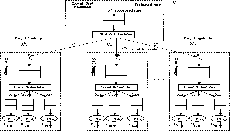
Figure 2. A Local Grid Manager Queueing Model

• VI.    Simulation Results and Discussion

• A.    Simulation Tool and Environment

Even though there are many available tools for simulating scheduling algorithms in Grid computing environments such as Bricks, OptorSim, SimGrid, GangSim, Arena, Alea, and GridSim, see [27] for more details, the simulation was carried out using the GridSim v4.0 simulator [28]. It provides facilities for modelling and simulating entities in grid computing environments such as heterogeneous resources, system users, applications, and resource load balancers which are used in designing and evaluating load balancing algorithms. In order to evaluate the performance of the proposed load balancing policy, a heterogeneous grid environment was built using different resource specifications. The resources differ in their operating systems, RAM, and CPU speed. In GridSim, tasks are modelled as Gridlet objects which contain all the information related to the task and the execution management details. All the needed information about the available grid resources can be obtained from the Grid Information Service (GIS) entity that keeps track of all resources available in the grid environment.

All simulations experiments have been performed on a PC (Dual Core Processor, 3.2 GHz, 2GB RAM) running on Windows xp OS. The bandwidth speed between LGMs (low capacity link) was set to 10Mbps, and the bandwidth speed between LGMs and SMs (high capacity link) varies from 50Mbps to 100Mbps. All time units are in seconds.

• B.    Performance evaluation and Analysis

Both of the external (remote) tasks and local tasks arrive sequentially to the LGMs and the SMs respectively with inter-arrival times which are independent, identically, and exponentially distributed. Simultaneous arrivals are excluded. The service times of LGMs are independent and exponentially distributed. Task parameters (size and service demand) are generated randomly. Each result presented is the average value obtained from 5 simulation runs with different random numbers seeds.

Experiments 1:

On a heterogeneous grid model consisting of 3 LGMs having 4, 2, 1, 5 SMs respectively. The total grid processing capacity is set to 1000 task/second (t/s). For this model to be stable, total task arrival rate (remote arrivals plus local arrivals) must be less than 1000 t/s. In this experiment, we focused on the results related to objective parameter (i.e., overall mean task response time) according to various numbers of tasks. During the experiment, 20 % from the total tasks arrived to the SMs are local tasks. In Fig. 3, we compare between the grid overall mean task response time obtained under the proposed load balancing policies (PLBPs) and that obtained without using any load balancing policies at all (No. LB). From that figure, we can see that as the number of tasks increases the overall mean task response time increases. The increase of grid overall mean task response time is less in PLBPs as compared to the increase in the grid overall mean task response time without using any load balancing policies.

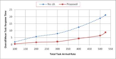
Figure 3. Grid overall mean task response time of PLBPs vs. No. LB

To evaluate how much improvement is obtained in the grid overall mean task response time as a result of applying the PLBPs, we computed the improvement ratio (T - T )/T , where T is the grid overall mean task response time without using any load balancing polices, and T _P is the grid overall mean task response time under PLBPs, see Fig. 4. From that figure, one can see that the improvement ratio gradually decreases as the grid workload increases, and it decreases rapidly as the grid workload approaches the saturation point (i.e., traffic intensity (^/ц)~1). The maximum improvement ratio is about 73% and is obtained when the grid workload is low. This result was anticipated since the PLBPs distribute the grid workload based on the resources occupation ratio and the communication cost which leads to maximizing grid resources utilization and as a result the grid overall mean task response time is minimized. In contrast, the distribution of the grid workload on the resources without using any load balancing policies (No. LB.) leads to unbalanced workload distribution on the resources, which leads to poor resources utilization and hence, the grid performance is affected.

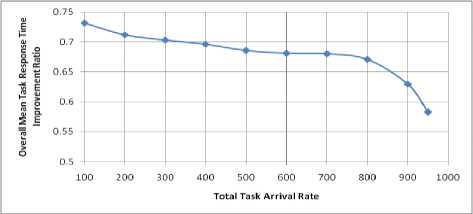
Figure 4 Grid overall mean task response time improvement ratio

Experiments 2:

In this experiment, the performance of the PLBPs is compared with that of Random_GS and Random_LS policies described in [22], and Min_load and Min_cost policies described in [13]. Our model is limited to approach their models by reducing the number of LGMs to 1 and setting the Local Tasks Arrival Rate (LTAR) to 0 (i.e., no local arrivals is allowed). In this case the LGM represent the Grid Manager (GM) or Global Scheduler (GS) in their models. During the experiment, we set the number of SMs to 4 with total processing capacity of 550 t/s. For this model to be stable, external arrival rate must be less than 550 t/s. Each simulation ends after 550,000 tasks are completed. Fig. 5 shows the overall mean task response time obtained under the Random_GS and Random_LS, Min_Load and Min_Cost, and the proposed load balancing policies. From that figure, we can see that the grid overall mean task response time obtained by all policies increases as the total arrival rate increases. Also from that figure, we can see that the PLBPs outperforms the Random_GS and Random_LS, and Min_Load and Min_Cost policies in terms of grid overall mean task response time.

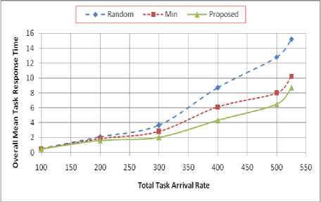
Figure 5. Grid overall mean task response time of Random_GS and Random_LS, Min_Load and Min_Cost, and the proposed load balancing policies.

To evaluate how much improvement is obtained in the grid overall mean task response time as a result of applying the PLBPs over the other policies, we computed the improvement ratios (T - T )/T , and (T _M - T _P )/T _M where T _R , T _M , and T _P are the grid overall mean task response time obtained using the Random_GS and Random_LS, Min_Load and Min_Cost, and the PLBPs, see Fig. 6. From that figure, one can see that the PLBPs outperforms the Random_GS and Random_LS, and Min_Load and Min_Cost policies in terms of grid overall mean task response time and the maximum improvement is bout 50% and 30% respectively. The improvement ratio gradually increases as the grid workload increases until the workload becomes moderate where the maximum improvement ratio is obtained and after that the improvement ratio decreases gradually as the grid workload increases approaching the saturation point (i.e., traffic intensity W)

This result was anticipated since the PLBPs distribute the grid workload based on the resources occupation ratio which leads to maximizing the resources utilization and as a result, the grid overall mean response time is minimized. In contrast, the Random_GS and Random_LS load distribution policies distribute the workload on the resources randomly without putting any performance metric in mind which may lead to unbalanced workload distribution. This situation leads to poor resources utilization and hence, the grid performance is degraded. Also, Min_Load and Min_Cost load balancing policies suffer from higher communication cost compared to the PLBPs. Notice that in the PLBPs, once a task is accepted by a LGM, it will be processed by any of its sites and it will not be further transferred to any other LGM. In contrast to the Min_Load and Min_Cost load balancing policies where a task may circulate between the grid resources leading to higher communication overhead. To be fair, we must say that according to the obtained simulation results, the performance of the Min_Load and Min_Cost load balancing policies is much better than that of the Random_GS and Random_LS distribution policies.

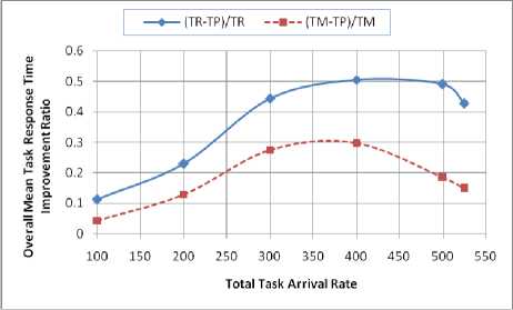
Figure 6. Improvement ratio obtained by the proposed load balancing policies over Random_GS and Random_LS, and Min_Load and Min_Cost policies.

Experiments 3:

This experiment is done to study the effect of the local arrival rate on the performance of the PLBPS. During the experiment, the same grid parameters setting of the second experiment is used, and we set the ratio of the LTAR=0% , LTAR=10% and 25% form the TTAR to the grid. As it can be seen form Fig. 7, the overall mean task response time decreases as the LTAR ratio from the TTAR increases. This result is obvious since the LTAR arrives directly to the SMs and don't suffer from any transmission delay at all.

♦ - LTAR=O% TTAR ••■■•• LTAR=10% TTAR   —*— LTAR=25%TTAR

Total Task Arrival Rate (TTAR)

Figure 7. Grid overall mean task response obtained for different ratios of LTAR from TTAR.

• VII.    Conclusion and future work

In this paper, we proposed a fully decentralized two-level load balancing policy for balancing the workload in a multi-cluster grid environment where clusters are located at administrative domains. The proposed load balancing policy takes into account the heterogeneity of the grid computational resources, and it resolves the single point of failure problem which many of the current policies suffer from. The load balancing decisions in this policy are taken at the local grid manager and at the site manager levels. The proposed policy allows to any site manager to receive two kinds of tasks namely, remote tasks arriving from its associated local grid manager, and local tasks submitted directly to the site manager by the local users in its domain, which makes this policy closer to reality and distinguishes it from any other similar policy. It distributes the workload based on the resources occupation ratio and the communication cost which leads to minimize the grid overall mean task response time. To evaluate the performance of the proposed load balancing policy a simulation model is built. In this model, the grid overall mean task response time is considered as the main performance metric that need to be minimized. The simulation results show that the proposed load balancing policy improves the grid performance in terms of overall mean task response time.

In the future, we will try to study the effect of the length of information update periodical interval at the GS and LS on the performance of the proposed load balancing policy. Also, we will try to increase the reliability of the proposed policy by considering some fault tolerance measures.