A Host-Vector SIR Model for Diarrhea Transmission: Analyzing the Role of Houseflies in Bangladesh

Mathematical modeling has become indispensable in understanding infectious disease dynamics and designing effective interventions. Compartmental models such as SI, SIS, and SIR remain foundational frameworks, providing a structured way to quantify transmission, recovery, and intervention impacts. These models allow researchers to explore disease persistence, eradication, and the effectiveness of public health strategies. Their applications range from influenza and HIV/AIDS to diarrheal diseases and, more recently, COVID-19, where they have informed policy decisions by estimating transmission potential, intervention thresholds, and herd immunity effects.

Early research primarily focused on theoretical development and model validation. Kandhway and Kuri [1] demonstrated optimal control strategies for SIS and SIR dynamics, highlighting how interventions can be timed to minimize spread. Rodrigues [2] provided a comprehensive analysis of the classical SIR model, emphasizing its versatility for various infectious diseases. Ehrhardt et al. [3] extended the SIR framework to incorporate vaccination and waning immunity, applying numerical methods to examine disease progression, while Zaman et al. [4] analyzed equilibrium states to distinguish conditions leading to disease-free or endemic populations. Barro et al. [5] integrated time delays with optimal control, bridging theoretical modeling and applied intervention strategies. These studies collectively underscore the importance of connecting mathematical rigor with practical epidemiological interpretation.

Subsequent research has adapted these models to disease-specific contexts, particularly diarrhea, which involves complex interactions between human populations and vectors such as houseflies. Rahmadani et al. [7] developed a multi-compartment model including vectors to evaluate ten control scenarios, illustrating how vector dynamics can shape disease outcomes. Affandi and Salam [8] adopted an SIR-VT model incorporating vaccination and treatment, optimizing interventions using numerical simulations. These studies demonstrate the potential of SIR-based models to inform resource allocation and intervention design but also reveal a recurring limitation: most rely on estimated parameters rather than robust empirical data, limiting real-world validation [10-13].

Recent modeling efforts emphasize heterogeneity, stochasticity, and delay effects to enhance realism. Zhang et al. [15] introduced fixed infectious periods as delays in SIR dynamics, capturing realistic temporal progression of infection. Acemoglu et al. [19] developed a multi-risk SIR model, showing that age-stratified infection and mortality risks critically influence disease outcomes. Sharif et al. [22] incorporated stochastic environmental fluctuations in diarrheal disease models, providing insights into persistence, extinction, and long-term dynamics under uncertainty. These advancements highlight the growing sophistication of epidemic modeling in accounting for real-world complexity. Despite these contributions, several gaps remain. Most studies emphasize mathematical or computational results without integrating empirical epidemiological data, which limits parameter validation and predictive accuracy. Furthermore, the literature often lacks comparative evaluation of modeling approaches, with limited discussion of how assumptions (e.g., homogeneous mixing, constant populations, or vector behavior) affect results. Finally, there is insufficient linkage between mathematical findings and actionable public health strategies in specific regions, reducing the practical relevance of many models [23-27].

Addressing these gaps, the present study develops a computational SIR model for diarrhea that integrates realistic assumptions, interprets equilibrium points epidemiologically, and evaluates intervention strategies in regions such as Khulna and Jashore. By combining theoretical rigor with empirical plausibility, this work provides insights into disease dynamics that can inform targeted public health interventions and contribute to broader efforts in diarrhea control and eradication.

The paper is organized as follows: Section 2 reviews the classical SIR model by Kermack and McKendrick; Section 3 introduces the proposed SIR model for diarrheal disease; Section 4 presents results and discussion; and Section 5 concludes with key findings and future directions.

2.    Methodology 2.1    SIR Model Due to Kermack and Mckendrick

In this part, we will discuss a fundamental SIR model [25]. It is used to simulate the spread of various infectious diseases within a large population. The population is divided into three groups, identified by the labels s , I and R . Each of these is a function of time t .

• ∎ S represents the number of susceptible individuals who are not currently infected but are at risk of becoming infected.

• ∎ Ф denotes the rate of infection. Susceptible individuals become infected through interactions with infective individuals.

• ∎ I indicates the total number of infected individuals. These individuals carry the disease and are capable of transmitting it to susceptible.

• ∎ R represents the recovery rate. Infected individuals recover over time.

• ∎ R represents the number of individuals who have been removed.

  

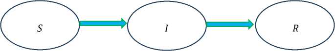
Fig. 1. Basic SIR model diagram

The transmission of infection depends on the interaction between susceptible and infected individuals. New infections result from contact between susceptible individuals and those who are infective. In this model, the rate of new infections is given by SI , where Y is a positive constant.

When a new illness arises, the affected individual moves from the susceptible to the infective class. There are no other mechanisms in this approach for individuals to transition in or out of the susceptible class. The alternative procedure involves transferring infective individuals to the removed class. It is assumed that this happens at a rate of I, with № being a positive constant.

as _ ysi

=-

Through the model, we assume the total population remains constant. The population is made up of susceptible, infected, and recovered individuals. Total population: N =( S + I + R ).

3.    SIR Model for Diarrhea Disease

Though the SIR model is primarily used to evaluate stability of disease in human populations, it is equally applicable to vectors. The transmission of diarrheal disease to humans occurs via contact with houseflies ( f ) . This effect needs to be represented within the SIR model. The recovery rate of houseflies will be overlooked because of their limited lifespan.

Let H ^ denote the total human population, including susceptible, infected, and removed individuals( S^ , I , Rh ). Again, let F_v denote the total vector population, consisting of both susceptible and infected houseflies( Sv , I_v ). In this model, H h and F_v are considered to be constant. As a result, the birth rate for the total population is S к^к , where к refers to either V (vectors) or ℎ (host), and ^k is the corresponding death rate.

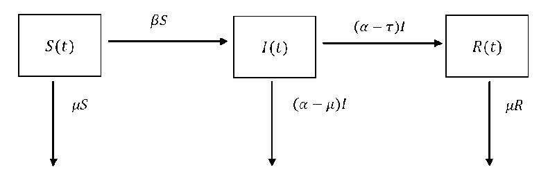
Fig. 2. Schematic diagram of diarrhea infection transmission

Description of variables and parameters of this model:

∎ s ( t ) be the number of susceptible individuals at time t .

∎ I ( t ) be the number of infected individuals at time t .

∎ R ( t ) be the number of recovered at time t .

∎ a be the constant recovery rate.

∎ ft be the rate of contact that is sufficient to transmit the disease.

∎ d be the death rate due to diarrhea disease.

∎ µ be the rate of natural death.

∎r be the rate at which infected people are recovered.

∎ H h represents the total human population.

∎ Sh represents the number of humans who are susceptible, meaning they are not infected but could potentially become infected.

∎ ^h represents the number of infected humans. These individuals are infected with the disease and have the ability to transmit it to the houseflies.

∎ Rh denotes the total number of human individuals who have been removed. These individuals may or may not carry the disease, but they are unable to infected again or transmit it to others. These individuals could have natural immunity, recovered from the illness with immunity, be infected but unable to spread it (due to isolation), or may have died. This mathematical model makes no distinguish among these options.

∎ Sh denotes the birth rate of humans. The parameter interacts directly with the overall population H h .

∎ ^h represents the human death rate.

∎ Ip h represents the human infection rate.

∎ Rh represents the human recovery rate.

∎ F_v represents the total population of houseflies.

• ∎    S_v represents the number of houseflies that are susceptible, meaning they are not infected but have the potential to become infected.

• ∎    I_v represents the number of houseflies that are infected. These infected houseflies have the disease and can spread it to humans.

• ∎    фр represents the infection rate for houseflies.

• ∎    ^v represents the death rate for houseflies.

• ∎    S_v represents the birth rate for houseflies. The parameter interacts with the overall housefly population Fv .

• ∎ f denotes the average interaction rate of a housefly.

First, we will determine the host model, which describes the rates of susceptible, infected and recovered human. The interaction model is described by three differential equations.

dish =     - ^ Ivsb - Eh^h(4)

diIh =        -(Eh + Uh) Ih(5)

dt =     - £h^h(6)

Next, we will determine the vector model, which describes the rates of susceptible and infected vectors. The interaction model is described by a system of two differential equations.

=     - „ hi$v - ^V^v(7)

=        - ^v^v(8)

Now, we may also consider that ^h =   , £_v =   , therefore we have these two models as follows:

dtsh =     - ^ Ip^h - ShSh(9)

=        -(Sh + Uh) Ih(10)

dt =     - 8hRh(11)

and

=     - „ Ih^v - 8VSV(12)

at I” =         - sviv(13)

Since total human population is equal to the addition of susceptible, infected and recovered individuals, so we have,

$h ⁺ Ih ⁺ Rh =   ⇒ Rh =    ^- Rh ^- Ih

Again, since total vector population is equal to the addition of the susceptible and infected individuals, so we have, s+I=  ⇒s=-

+ = ⇒ =

In order to comprehend the stability of human and housefly populations, it will reorganize both models and combine them into one.

Applying (14) to (11)

d

⇒  (Hh at

-

d dt ^^ =    - RhRh

sh

-

Ih ) = ^hlh ^- ^( Hh

-

Sh

^- Ih )

⇒

Applying (15) to (12)

⇒0-  -  =   -   +   +

I IL IL                          IL IL         IL IL at at

⇒-  =   -   +   +   +

I IL IL         IL IL         IL IL         IL IL clt                                        at

- ^ = fi_hI_h - 8_hH+ + 8_hS_h + 8_hI_h + 8_hH_h —^I_vS_h - 8_hS_h [ using(9) ] dlh

⇒-  =   +- atn^

dlh

⇒   =       -(  +)

at ^

⇒

=   -- at^

d

(  - )=    -       -( dl„

⇒0-  =-+ at ti h

-  )

dlv_

⇒   =     -

As a result, these two equations tell us that our conditions can be expressed as,

=    -      -

=      -(  +  )

In order to simplify the model by removing its nonlinear terms, we will nondimensionalize it.

()=  ; ()=  ; ()=

Let us define,

×                     ×

~ H_h ~                        total human population

• •    = = ( 8_h + fl_h) = Birth rate of human + Recovery rate of human;

• •    fi = f tp_v = Average of housefly contact x Infection rate of houseflies;

• •   =   = Birth rate of houseflies;

• •   =   = Birth rate of human;

Thus, we get from (16)

( )=    -- atn h

( )

⇒  ( )=  -- dx            ibhfI„F„

⇒    =   - ( )        -(t)

atn *v lbhfFv

=   -  ( ) ( )       -( )

=  {1- ()}-() ()

Equation (17) becomes

From (18)

(4) = ^ЛА at       n ^

^-(^} = dt \Hh)

^   = x( t)

—

^hf^hJv

HhHh ^hf^v Fy

Hh

= x(t)z(t)

—

( 8_h +F J4

( 8 ^ + FJ^

—

; Fy TphfPy

Hh

⁽⁸и + FuM О

^— уу⁽ 0

= cx( t)z(t) —уу( t)

^ly =    Ih—-8VIV d ly   ipvfIftPy   8VIV

^   =      — dt Fv HhFv Fv dz        F^y

^ =У«)^ — ( z(t)

—

= y^F—^--Zz( t)

= yC^FC— — z⁽O} — <ХО

Thus, by nondimensionalizing the system, we obtain the following model:

= 8{1 — x(t)} — xx()W)	(20)
= xx(t)z(t) - yy(t)	(21)
^ = y(t)F{1 —z(t)} —	(22)

To identify the point(s) of equilibrium, the aforementioned equations must be set to 0. Therefore,

^ = 8{1 —x(t)} —^(tW)^

= Ex(t)z(— — yy{t)       = 0 ■

^ = y(tFF {1 — z(t)} — Z(t t) = 0,

Solving this system yields two equilibrium points. The first (1,0,0) represents the Disease-Free Equilibrium (DFE), where no infected humans (y = 0)or vectors(z = 0) exist, and the entire human population is susceptible (x = 0). The second ( , , ) represents the Endemic Equilibrium (EE), where the disease persists in the population at a constant level.

г = ^Л A

⁰ H (5+г)

_ 5 te-rf)

0    № G5+£)

• ₇ _ S ⁽u г - 1O

' ⁰ = г(_м 5+1O 7

Let, у = —,y = ^,W = — (it dt          dt

Now, using the Jacobian of the non-dimensionalized model, we obtain the following,

J ( X ^, У ^, z )=

I ^-s

-

ez

⇒ J ( X , У , z )=

EZ

⎝  0

/dU

I dx

dW

\ dx

V

dU dy

dW

dy

^- У

-

ZU

dU\ dz \

dV dz

dW dz /

-

- EX \

EX

So, at the equilibrium point (1,0,0), we obtain

J (1,0,0) = ⎜	- 6      0 0- У ⎝0      V	- ' ⎞ £ - < ⎠	⎟                                             (26)
To find the eigenvalues, we set
- S - л	0	- £
|      0	- У - л	Е	|=0                       (27)
0		-< -	-Л 1

This yield

The three eigenvalues are

⇒(- 6 - X )(- ЕЦ + Y^ + Y^ + ^X + Л²)=0                     (28)

Ai =- S

Аг ₌ (- У ^-< -√4 ЕЦ + У² -2к+ <²

Аз = (- У ^-< +√4 ЕЦ + У² -2К+ <²

}

negative.

We have ^1 and А 2 are always negative, because У ,с, /л are always positive and ^з can be either positive or

At the equilibrium point ( Xq , Уо , z₀), we have

	- 8 - Е ( 5- ( ^ ) ) Vг(М^+ГС)	0	- Е (М) V(3+£)	⎞
⎜ J ( %0 , Уо , Zo )= ⎜	Е ( 5- ( М^ ) ) V £( l^o+Y< )	- У	Е (М) V(3 + £))	⎟ ⎟⎟
	⎝ 0	- ( 5- ( ^ ) ) (М^+ГС)	- V ( s- ( ^ ) )- \ хи (3+£)	< ⎠

To find the eigen-values we set

8 - E ( &- ( ^ ) )- A \E( HS+Y^ )	0	f Sh+YZ \       1 - £(M(5+£))
E ( S- ( ^ ) ) V ( HS+Y^ ) )	- Y - A	E (M) Vm (5+£ ))	= 0        (31)
0	- (* ( ^ ) ) V( hS+yZ ))	- ( s- ( Л ; F ) )- c -A V ум (5+£)

The eigenvalues of the system can be efficiently computed through computer simulations, for which Maple provides an effective computational platform. In addition, assigning specific numerical values to the parameters facilitates a clearer stability analysis.

Reproduction Number Rq

The equilibrium point ( ^0 ,У о, Zq ) is meaningful only if Уо , Zq are positive. This depends on a threshold parameter, the basic reproduction number, ^0 given by:

Ло

ЕМ

О'

An epidemic occurs if ^0 > 1, and the disease dies out if ^0 < 1.

4.    Results and Discussions

In this section, we present numerical data based on the SIR model for diarrhea infection. Chaturvedi et al. [26] provided several parameter values intended to support further analytical and numerical studies. These values are summarized in Table 1. Using this dataset, together with supplementary information from additional sources, we conduct a series of simulations to investigate the model’s dynamical behavior.

Table 1. Basic parameters

Name of the Parameter	Symbol	Initial Value
Transmission probability of vector to host	фр	0.5
Transmission probability of host to vector	Фл	0.2
Contacts per susceptible housefly per day	fs	0.4
Contacts per infectious housefly per day	fl	0.6
Interaction Rate, Host to Vector	Clw	0.5
Interaction Rate, Vector to Host	Cvh	0.3
Human Life Span	1	HL
Vector Life Span	1	VL
Host Infection Duration [33]	1 + Hh       \	5 Days

HL and VL represent the life span we obtained from resources. Let us consider analyzing the population of Khulna city in Bangladesh. Record shows that Khulna city has total population of 10, 00,000 [28]. Therefore, we consider some parameters for this population and assume there are 300,000 houseflies in Khulna [22]. Let us consider HL = 26650 days [29] and VL = 25 days [30] are regarded as the minimum lifespan of a housefly.

Now we have,

^ _ ГФк^ _ s=  = n HL

о.6×О.2×300000

= 0.036 1000000

=     = 0.0000375

I =  =

.

1       1

=   = 0.04

VL 25

№ =    =0.6×0.5 =0.3

Y =( S_h + Ин )=| = 0.2

Now putting the values of € , 8 ,(, /л and у , into (24), we get,

Su + XL n ( s + E )

s ( ЦЕ - Xi ) YU ( S ⁺ E) S ( ЦЕ ^- Xi ) E( цЗ + Y( )

(0.0000375 × 0.3) + (0.2 × 0.04) 0.3 × (0.0000375 + 0.036)

= 0.74101

0.0000375 × (0.3 × 0.036 - 0.2 × 0.04) (0.2× 0.3) × (0.0000375 + 0.036)

0.0000375 × (0.3 × 0.036 - 0.2 × 0.04) 0.036 × (0.3 × 0.0000375 + 0.2 × 0.04)

0.0000486

0.000364

Thus, the equilibrium points are:

( S_h , X , R_h ) = (1,0,0) and ( s_h , X , R_h ) =(0.74101, 0.0000486, 0.000364 )

Now, we need to calculate the eigen-values for the equilibrium point (1,0,0).

From (29), we get three eigen-values. That are,

Ai =- s

Аг = (- Y ^-< -√4 ЕЦ + Y² -2 Yt + <² )

A3 = (- Y ^-< +√4 ЕЦ + Y² -2 Y( + <²)

Now putting the values of € , 8 , ( , n and Y , we get,

Ai = -0.0000375 = -0.251149 Л = 0.011149

Therefore, we get the eigen-values for the equilibrium point, (1,0,0) are: ^1 = -0.0000375,     ⁼

-0.251149 andA 2 = 0.011149, which is unstable, as the eigenvalue ^3 is positive. This result aligns with our finding that R_o >1, predicting that the disease-free state is not sustainable.

Again, we need to calculate the eigen-values for the equilibrium point (0.74101, 0.0000486,0.000364 )

Now, based on the Jacobian of the nondimensionalized model from (25), we have

/ - s - EZ		0	- EX \
J ( X , У ,Z)=⎜		- Y	“ ⎟
	⎝0	I1 - гц	- ^y - ⎠

At the equilibrium point (0.74101,0.0000486,0.000364 ),

	/-0.0000244	0	-0.026676 \
J (0.74101,0.0000486,0.000364) =⎜	0.0000131	-0.2	0.026676  ⎟ ⎟
	⎝0	0.299891	-0.0400146⎠

To find the eigen-values we set

-0.0000244 - Л	0	-0.026676
| 0.0000131	-0.2 - Л	0.026676	=0
0	0.299891	-0.0400146 - Л 1

Using Maple software, the eigenvalues of the equilibrium point, (0.74101, 0.0000486, 0.000364 ) were computed as Ai = -0.2400038 , a₂ = -0.0000176 + 0.000661 i and = -0.0000176 - 0.000661 i . Since all eigenvalues have negative real parts, the equilibrium is stable. This result corroborates our finding that, with a basic reproduction number ^o = 1.35, the disease cannot be eradicated and is expected to persist in the population, becoming endemic.

Also, from equation (32) we get the basic reproduction number:

0.036 × 0.3

^{=   =} 0.04 × 0.2 ^{= 1.35}

Since = 1.35 > 1, the disease is expected to persist and become endemic in the population.

• 4.1.    Sensitivity Analysis

To identify the most critical parameters for disease control, we performed a sensitivity analysis on . We varied each parameter by ±25% while holding all others constant at their baseline values and recorded the change in .

Table 2. Basic parameters and sensitivity analysis

Parameter	Description	Baseline Value	(Value +25%)	(Value -25%)
£	Vector-to-Host Rate	0.036	1.688	1.013
A	Host-to-Vector Rate	0.3	1.688	1.013
g	Vector Death Rate	0.04	1.08	1.80
Y	Human Recovery Rate	0.2	1.08	1.80

The sensitivity analysis reveals that R ₀ is most sensitive to changes in the human recovery rate (y ) and the vector death rate ( g ) • This suggests that interventions focused on treating infected humans (to increase у ) and controlling the housefly lifespan (to increase g ) will have the most significant impact on reducing the spread of diarrhea.

We will now create two cases based on these parameters.

Case I:

Let us assume some initial data. Consider the case where we have (0) = 53000,   (0) = 25500,   (0) =

• 0, and (0) = 50000, ,  (0) = 25000 [31]. Based on the initial data, we get the following table.

Table 3. Simulation results for Case I in Khulna city

Days	Sh ( t )	Ih ( t )	Rh ( t )	Iv ( t )
0	53000	25500	0	25000
10	34000	16000	15000	16000
20	26000	8500	26000	11500
30	19000	3000	31000	6000
40	13000	2000	35400	4800
50	9000	1000	37000	2500
60	7500	850	38100	1050
70	5200	470	39300	500
80	3100	280	40500	420
90	2300	0	41000	280
100	1500	0	42500	0

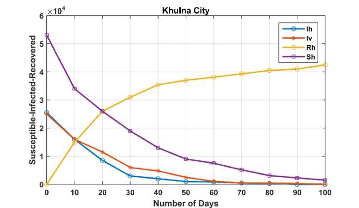
Fig. 3. Temporal dynamics of human and housefly populations in Khulna city for Case I

The graph indicates that a significant portion of the population recovers over time, with time measured in days. The simulation shows that the number of infected humans approaches zero after approximately 90 days, while the population of infected houseflies reaches zero around day 100. Notably, some susceptible individuals remain uninfected by day 100, as there are no longer any infected houseflies to transmit the disease. Consequently, the numbers of susceptible and recovered individuals stabilize by this time, which aligns with expected epidemiological behavior.

Case II:

Let us assume some initial data. Consider the case where we have (0) = 64000,   (0) = 21500,   (0)=

0, and (0) =90000,,  (0) = 19000 [32]. Based on the initial data, we get the following table.

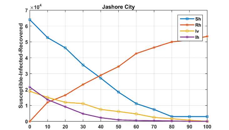
Table 4. Simulation results for Case II in Jashore city

Day	Sh ( t )	Ih ( t )	Rh ( t )	Iv ( t )
0	64000	21500	0	19000
10	52700	13700	12000	15100
20	46300	9200	16500	12000
30	35480	4800	23200	11200
40	27200	2300	29000	7500
50	18400	950	34500	6200
60	11200	560	42700	4700
70	7500	420	46500	2500
80	3000	250	50000	1650
90	3000	0	51200	720
100	3000	0	53500	0

Number of Days

Fig. 4. Temporal dynamics of human and housefly populations in Jashore city for Case II

The graph illustrates that a significant portion of the population recovers over time, with time measured in days. The simulation indicates that the number of infected humans approaches zero after approximately 85 days, while the infected housefly population reaches zero after about 100 days. Notably, since there are no remaining infected houseflies, some exposed individuals remain uninfected beyond day 100. Consequently, the numbers of susceptible and recovered individuals stabilize after this period, consistent with expected epidemiological behavior. Furthermore, the results suggest that highly infected houseflies die at a faster rate than those with lower infection levels, highlighting the impact of infection intensity on vector mortality.

5.    Conclusion

This study successfully developed a host-vector SIR model to analyze diarrhea transmission in Bangladesh. By establishing a system of five ODEs and non-dimensionalizing them, we established two key equilibrium points: the Disease-Free Equilibrium (DFE) and the Endemic Equilibrium (EE). Our primary finding is the calculation of the basic reproduction number, = 1.35, for Jashore and Khulna city. This critical value, being greater than 1, demonstrates that diarrhea is not a temporary outbreak but is endemic in the region. This mathematical result is consistent with the stability analysis, which showed the DFE to be unstable and the EE to be stable. The results emphasize the importance of considering both human and vector dynamics in modeling diarrheal diseases and provide a quantitative basis for public health interventions. By highlighting the persistence of the disease and the key factors driving its transmission, this study offers valuable insights for the design of targeted control strategies, such as vector management and improved sanitation measures, to mitigate the burden of diarrhea in affected communities.

6.    Public Health Implications

The goal for public health officials is to implement strategies that reduce the reproduction number to R₀ < 1. Our model's formula, R ₀ = ^, provides a clear guide for intervention:

• 1.    Reduce E (Vector-to-Host Transmission): £ is a product of fly contact rate ( f ) and human infection probability ^ ) . Public health campaigns should focus on vector control (e.g., insecticides, fly traps) to reduce the housefly population ( f ) and physical barriers (e.g., window screens) to reduce contact.

• 2.    Reduce ^ (Host-to-Vector Transmission): ^ is a product of fly contact rate ( f ) and vector infection probability ^ ) . This can be achieved by improving sanitation (e.g., building covered latrines, managing waste) to reduce the ability of houseflies to come into contact with infectious human material.

• 3.    Increase y (Human Recovery Rate): y is the sum of the human birth/death rate ( ^ ) and the recovery rate ( ^ ) . Increasing access to rapid medical treatment (e.g., rehydration therapy, clean water) will increase ^_h , which in turn increases y and lowers the R ₀ .