A Hybrid Approach for the Multi-sensor Patrolling Problem in an Unknown Environment with Obstacles

Published Online October 2020 in MECS DOI: 10.5815/ijcnis.2020.05.02

The world is facing increasingly severe disasters like forest fires, floods, earthquake, tsunamis and nuclear explosions. More concretely we can mention for example the natural disaster that occurred in Taiwan in February 2016 due to a violent earthquake. This disaster caused more than thirty deaths. However, sixty hours after the catastrophe, precisely about three days after, there were still survivors. Thus, the environment has long been regularly inspected by rescuers to detect other survivors. Usually, after this kind of disaster, the demarcated area is very hostile to the humans who move there. Therefore, several tools can be used to monitor such areas, including sensors, and thus sensor networks. Indeed, because of the advantages that they promise in terms of flexibility, cost, scope, robustness and even mobility, the sensor networks make it possible to solve the problems of monitoring and prevention. In fact, the purpose of a wireless sensor network is to monitor and control different events (or phenomena) in different environments [1]. Talk about monitoring by a small number of moving entities requires regular navigation in certain critical areas of the environment; which is akin to a patrol task.

The patrol problem depends on whether the environment is known or unknown. In a known environment, patrol agents are deployed with the environmental map to monitor; that is, all the domains they have to monitor during their task. By cons, in an unknown environment, it is impossible to have the map of the environment. Approaches based on pre-knowledge of the environment rely on the offline research of an optimal multi-agent path, which is then applied to the environment under consideration. Thus, they are unable to adapt to online changes in the problem such as the loss of an agent, the addition of an agent, the moving of an obstacle, etc. Moreover, very often, after a disaster, the aspect of the environment is unknowable. Therefore, in our work, we hypothesize that the environment is unknown for patrol agents.

The main problem we are interested in is the regular monitoring of all accessible places in an unknown environment by mobile and wireless sensors. We can take an example to explain it: monitoring a forest for signs of possible bush fires. Suppose the forest is divided into 2 zones. An agent was deployed to monitor them. The agent monitors zone 1 for 5 seconds; then he goes to zone 2 and monitors it for 15 min. Between 5 seconds and 15 minutes many things could have happened in zone 1. A bush fires may already be underway. However, if the agent had not taken enough time in zone 2, he could have returned to carry out a control in zone 2 and detect the telltale signs of a possible bush fire to come, in order to see how to prevent or contain the disaster. So, the purpose of this regular monitoring is to ensure the detection as quickly as possible of different events that may occur in the environment, avoiding static and dynamic obstacles. It is assumed that the communications are bidirectional and direct between the sensors and the base station.

Previous work on this problem has been carried out by other researchers. However, the results of these approaches in terms of idleness can be further improved in the sense of minimization. In addition, these proposed approaches are subject to drawbacks such as the local minima and the oscillations that we explain in the rest of this article. Also, outside the approach of [13], obstacle avoidance is not taken much into account in previous patrol algorithms; But this approach too is subject to local minima and oscillations.

This is why we propose to develop an approach allowing the sensors to regularly visit the areas of their environment, while avoiding any obstacles encountered during their navigation.

In order to successfully complete the obstacle avoidance phase, a learning process can be integrated into the sensors. In wireless sensor networks, there are generally three types of learning, namely supervised learning, unsupervised learning and reinforcement learning, [2].

Reinforcement learning (RL) can be defined as a problem of learning from experiences, the action to be taken for each situation, in order to maximize a digital reward over time. The optimal decision-making behavior of the learner is modeled as a strategy that associates the current action with the current state. Reinforcement learning therefore aims to generate from experience (current state, action, next state, reward) a policy maximizing local reward obtained as a result of an action on the environment, or maximizing on average the sum of rewards over time.

In addition, reinforcement learning, based on the paradigm of trial and error, called Q- learning [4], falls between supervised and unsupervised learning. It does not receive for each data x (state of the system), a label y (best action to perform) that must be associated with it. However, a local assessment called reward is provided for each pair (x, y) indicating approximately the quality of that choice. Thus, the agent is active by the choice of the couple state actions he will test and the R reward he will award. This notion of test for (x, y) and errors for R is specific to reinforcement learning.

As part of our work, this learning method is used to help the sensors in case of blocking situation between obstacles, to choose the best direction to get out of the blockage, without collision with the obstacles.

To solve the problem, we propose a hybrid approach called PREFAP. This approach has three components: a perception-reaction module, a module implementing a model based on forces for obstacles’ avoidance and a module integrating learning process. The rest of this work is organized as follows: section 2 presents a state of the art on the issue of the patrol; Section3 describes a hybrid approach to solving the problem. After a simulation of this approach, we will present in section 4 the results obtained and interpretation of these results in section 5. This work ends with a conclusion and perspectives in section 6.

2.    Related Works

Patrol: The multi-agent patrolling problem consists in making that agents cover a territory, so that different parts of the territory are visited as often as possible by these agents [2,3]. In [4], a multi-agent patrolling is defined as the act of effectively monitor an environment with a group of agents to ensure its protection. According to [4] Patrolling effectively in an environment, possibly noisy and dynamic, requires:

• –    minimize the time between visits to the same place,

• –    in the case of a monitoring mission, the members of a patrol should preferably follow unpredictable paths by agents wanting to infiltrate the area patrolled.

The problem of the patrol can be defined as in [5,6,7] as follows: Let G an environment, a number n of agents with limited perception with aim, regular visits of all available places or regions G. The main goal is to minimize the time between visits to the same place or the same region. In unknown environment, assume an impossibility for patrol officers to have the graph of the mapping of the environment. Thus, the environment G is represented by a cell matrix in which each cell can be free, busy or unreachable.

Patrol ’ s strategy [2, 7, 8, 9]: We will call a patrol strategy of the agent j, the function π : N → V such that π (j) is the j-th node visited by the agent. We denote by Q = { π , π } the multi-agent strategy, defined as the set of strategies π , π of r agents. ∏ r (G) denotes the set of possible multi-agent strategies with r agents on the graph G.

Instant idleness of a node [2]: The idleness of a node i at time t, denoted It (i) is the elapsed time since the last visit of an agent on that node. By convention, at time 0, idleness of each node is zero.

From idleness of a node, you can build a variety of criteria to measure the idleness of the graph at a time. We can build the average idleness (Average Idleness, AIt (G)) and the maximum or worst idleness (Worst Idleness, WIt (G) ) [2]. We have:

AIt(G)= ^„Ш

WI^G) = maxievIt(i)(2)

From instant idleness, we define global idleness of Gas follows:

AIt(G) = 1lT=iAIt(G)

W IT(G) = max12 TWIt(G)(4)

The optimum patrol strategy n* on G is such that n* =argminn AIT (G) if the AI criterion is used and n* = argminn W IT (G) if the WI criterion is used [6]. Thus, the patrolling problem is to find an optimum patrol strategy that minimizes the average idleness or maximum idleness, also called worst idleness.

Machado and al. in [9] proposed two solutions based on two different parameters: reactive agents and cognitive agents. The reactive agents act according to their current perceptions. Each agent moves according to the nodes that are directly adjacent to it and have not been recently visited; because they lack planning or reasoning skills. Cognitive agents, on the other hand, can perceive the whole territory and move to a part that has not been visited for a long time using a shorter path algorithm.

Sempe studied in [10], the influence of disturbances on the activity of a group of robots. He takes the task of patrolling as an example of a collective task. For this purpose, he proposed a model: TheCLInG model (Local Choice based on a global basis), which relies on the propagation of information related to elementary tasks (visits) in a representation of the environment shared by the robots, making the assumption that the agents are reactive. The strategy is to provide local information that summarizes the overall state of the graph through the spread of idleness from one region to another. Thus, a region i will carry a propagated idleness OPi in addition to its individual idleness Oi.

Glad proposed in [6], an ant algorithm dedicated to the multi-agent patrolling in unknown environment: the EVAP model based on the deposition and evaporation of information. The special feature of this model is to exploit only the evaporation process. The idea is to mark the visited cells by a maximum quantity of pheromones q 0 , and to use the remaining quantity as an indicator of elapsed time since the last visit (which represents idleness). Thus, the behavior of the agent is defined by a gradient descent of this pheromone, that is to say a behavior leading the agent to move to the cell containing the least pheromones.

In their work, the authors of [11] developed a model called EVAW, for the cover and patrol problem in unknown environment. Instead of depositing a fixed quantity of pheromone, agents mark the cell by the current date. Idleness of a node is therefore given by the difference between the value of the marking and the current date. The EVAW model is defined as the EVAP model, but substituting the pheromone deposit by the marking of the current date. The agents do not know their environment and have no memory, they are only able to move to a neighboring cell, to mark their current cell and to perceive the marking of neighboring cells.

Authors in [12] developed an online multi-agent patrolling algorithm for large partial ob- servable and stochastic environment where information is distributed alongside threats in environments with uncertainties. While agents will obtain information at a location, they may also suffer damage from the threat at that location. Therefore, the goal of the agents is to gather as much information as possible while mitigating the damage incurred. To address this challenge, they formulated the single-agent patrolling problem as a Partially Observable Markov Decision Process (POMDP) and proposed a computationally efficient algorithm to solve this model. But better heuristic and algorithms that provide theoretical performance guarantees can be elaborated. On the other hand, the formulation is a basic model of Unmanned Aerial Vehicles (UAVs) patrolling under uncertainty and threats; The communication system of the agents may locally break down by suffering from harms or some agents may get destroyed due to cumulated harms.

Fute and al. in [13], proposed a multi-agent patrol strategy in an unknown environment applied to the environment exploration problem. They defined two behaviors for the patrolling agents: firstly, on the basis of a set of forces or field of potential, then secondly a behavior based on the decreasing gradient of pheromones deposited in the environment. The simulation of these two strategies allowed an evaluation of the worst and average idleness.

Others authors proposed in [14, 7] an algorithm to detect events using an Ant Colony Optimization approach (ACO) and multi-agent patrolling. The patrolling task is provided by a mobile sensors network using two strategies: all agents are located on the same node (non- dispersion) at the initial time, and the agents are dispersed over the graph. In this case, the minimization of Worst Idleness, Energy consumption and communicational Idleness are not compatible. It is therefore necessary to seek compromise solutions called Pareto Front. The ACO algorithm employs competitive colonies of ants: each colony tries to find out the best multi-agent patrolling strategy, and each ant of a colony coordinates its action with the other ants of the same colony to elaborate an individual agent’s patrolling tour as short as possible. Detecting and reacting some phenomena as fast as possible by a group of mobile sensors requires a patrol capacity that minimizes other criteria, namely the maximum communication time between the receiver and its base station as well as the total consumption of energy on the sensor network.

In [15], the authors considered the deployment of a wireless sensor network (WSN) that cannot be fully meshed due to distance or obstacles. Several robots are then charged to get close enough nodes to be able to connect and conduct a patrol to collect all the data in time. It has been shown to be fundamentally a single bounded vertex (CBSC) coverage problem. They exposed a formalization of the CBSC problem and proved that it was NP-hard and at least as difficult as the commercial traveler problem (TSP). Then they provided and analyzed heuristic methods based on classification and geometric techniques. The performance of their solutions is evaluated in terms of network parameters, robot energy, but also random and particular graph models. So, the environment here is a graph and it is a known environment.

3.    Hybrid Algorithm Prefap: Perception-reaction, Strength Model and Learning

In this section we describe how we proceeded to elaborate our contribution called PREFAP. The sensory field of a sensor is delimited by Moore’s neighborhood (8 cells that are directly adjacent to it). the only data provided to sensors prior to deployment is a defined set of points to delineate the boundaries of the environment to be monitored. The sensor can identify any object in its neighborhood. Thus, behavior based on the perception-reaction principle can be defined by drawing on the EVAW approach defined in [6]. The sensor perceives the cells of its neighborhood and their markings, chooses among the perceived cells, a free cell of date (marking) minimal, moves towards this cell, and marks it by the current date.

In order to equip the sensors with a behavior that avoids obstacles, we have added a model of force to this perception-reaction model. However, seeking to avoid obstacles, the sensor can become trapped in an area. He must fight alone to get out of this trap. For this reason, we have integrated into the sensors a learning module allowing them to break the deadlock.

• 3.1.    Perception-reaction model and the strength model

In this part, we present how the strength model is coupled to the perception-reaction model. The model of perception-reaction present two limitations: the conflicts and hesitations,due to purely reactive behavior of the sensor. Hesitations appear when in its vicinity, the sensor has two or more free cells with minimum dates. In this case, it randomly selects a cell to direct to. Conflict situations occur when two sensors desire to move to the same cell. These sensors, in this case will collide. They continue to perform the same movement and the same choices for a while until the next hesitation.

The sensors collided can cause extensive damage in case of loss sensors. This is why we have used, in addition to the perception-reaction model, a model based on a set of forces to avoid collisions between sensors and to improve the avoidance of obstacles. The model of forces used is based on that described in [13,14]. The perception-reaction is now used in both cases:

• –    Case 1: In the absence of static obstacles in the sensory field sensor

• –    Case2: In the absence of sensors in the communicational field of the sensor

When both conditions are not met, the sensor uses the strength model to calculate its next destination. The direction of the sensor is given by the resultant strength acting on it. In the case on this work, three strengths act on a sensor:

• -    the attractive force pulling the sensor to his next objective noted local F_ob] ,

• -    the resultant force of repulsion forces exerted by theperceived obstacles noted F_obSi ,

• -    the resultant force of repulsion forces exerted by the sensors in its communicational field denoted F_reP[.

  _–

  
  

the resultant force of all forces exerted on the sensors noted F .

The following notations are necessary for understanding the equations that will follow(equations 5 to 10).

• –   C i : sensor i,

• –   R comi : radius of the communication field of the sensor i,

• –   m i : mass of the sensor i,

• –   Q: number of sensors in the communication field of the sensor i,

• –  M: number of sensors perceived by sensor i,

• –   O k : obstacle k,

• –   Ob: goal of sensor. Following

  F =

  
  

  "E^-u ET^-l "E^ ^F obj + ^F obs _L + ^F rep _L

  
  
  
  

E" *

^F obj_t     ^ obj ^ l^b                                                      (6)

*

1 repL

У ° F *

^ j=i ¹ rep_tJ

"""""""""* ^F obS i

^ k=1 Fobs_lk

*

¹ rep_L j       ^uij *

E" *^m i

^Fobs tk      ^Т^ ' Ь,",*\ 2 ^к!

With δ ij ,δ obj , λ ik calibration’s constants and

""ki ⁽

' cos 6 ki

-sin O kt

sinQ kt

cosO ki

"""""""""*

)-1^

-T—* —-ГТ*.

Where O_ki = angle (C_lO_k,C_lOb)

This technique improves the previous one (perception-reaction) by eliminating collisions. However, two blocking situations are observed: local minima and oscillations. Local minima are observed when the sensor is trapped in a potential or force well. Thus, the resultant forces F is null. The oscillations are due to the passage of the sensor between several obstacles or in narrow areas. it does not move forward and it just goes back and forth between two cells. These blocking situations are a real problem because they do not allow the effective implementation of the exploration task. Hence the need to integrate a learning module to the sensors to escape traps.

• 3.2.    Learning module

The learning module which is the last component of our model, is described in this section. To solve blocking problems, we integrated a learning module into the sensors. The learningmethod used is inspired by reinforcement learning techniques. In this case, learning is for the sensor to explore new ways to overcome blocking problems. This learning is a form of learning by trial and error. The sensor tries to perform each possible action and analyzes its result in order to determine the actual action to be performed. Under the Reinforcement Learning Foundation, each try deserves a reward or reinforcement. The sensor analyzes the results of actions according to its rewards.

In each state, the sensor has eight (8) possible actions corresponding to the neighborhood of Moore. The state of a sensor is its position in the environment. When the sensor is in a state, it tries to perform the 8 possible actions. For each action, he receives a reward and chooses to perform the action that maximizes his reward.

One of the problems of reinforcement learning is the exploitation / exploration dilemma. Exploitation consists of reusing the tests carried out in certain states to decide on new actions. Exploration for its part consists in not using the old tests to discover new possibilities for action. In our framework, the exploitation can give a bad destination to the sensor since the state of a cell can change. A cell can be free at one iteration and be busy the next iteration or even inaccessible. That’s why we use exploratory learning to discover new opportunities.

Let Q: SXA → value, the utility function related to the actions. We chose to learn by Q-learning; that is to say to choose the action that maximizes the supposed usefulness Q(s,a) of action “a” in state “s”. This function is used to select the best action “a” to run in state “s”. It will be noted by the relation:

n(s) = argmaxQ(s, a)                                   (11)

The sensor receives a positive signal for a good action and a negative signal for poor action. A table of values is used for storing the values of Q (s, a) in order to determine the value of π(s).

We define by T: SXA → S, the transition function returning the new states’ obtained by performing the action “a” in the state “s”. If the action leads to a cell out of the environment, then s’ will be null. We have the following relationship.

s'= T (s,a)                                                (12)

However, determining the best action “a” for a state “s” based on the rewards received for each possible action in that state is a limitation. Indeed, the best action is just better in terms of rewards and may not be better in terms of idleness. This means that the best action can guide the sensor into a cell whose idleness is not maximal among the potential cells. Therefore, a Q-learning adaptation is necessary or rather redefining “Best action”. Thus, in our context “Best action” will not be the one that maximizes the reward of the sensor but the one that has a positive reward and leads the sensor to a cell that has not been visited or has taken long without receiving visits. Therefore, after having determined the values of Q (s, a), we choose among the actions which had a positive signal, one that leads the sensor towards a cell of maximum idleness. However, there may be several actions with positive signal, leading the sensor to a maximum idleness cell. In this case, the sensor will randomly select from among them, a cell to which to move.

Algorithm 1 gives an algorithmic description of the learning module of a sensor.

In this time, anymeasurementoriginates from clutter or falsehood.

The algorithm takes as input the initial state of the sensor as well as the set of possible actions in this state. It outputs the state obtained from the best action that can be performed by the sensor in its original state.

Qvalues store different values of Q(s, a) associated to the respective actions. Tvalues store the various values of T(s, a). After storing the values of Q(s, a), we store in Tvalues the values of T(s, a) for which Q(s, a) is positive. Each value is associated to the action concerned.

argmax(Tvalues) is the function that returns the action for which T(s, a) has a maximum idleness. The new sensor state is the result of this action. If this action is null, the new sensor state is the initial state.

Algorithm 1 : Learning’s algorithm of a sensor

Input : s , actions

Output : newEtat

Initializations :

Qvalues = 0

Tvalues = 0

newEtat = s act = null foreacha in actionsdo { add (a, Q(s, a)) in Qvalues

} foreacharg in Qvaluesdo {

}

}

If ( Tvalues is not empty)

{ act = argmax(Tvalues)

} newEtat = T(s, act)

Armed with this learning module, when the sensor is in a local minimum or oscillations, it will use its intelligence to successfully get out of these blocking issues. Similarly, if the strength module runs the sensor out of its environment, it will also use this learning to successfully remain in its environment.

• 3.3.    Algorithmic description of PREFAP

In this section we give the algorithmic description of the PREFAP solving approach. The sensor perceives its environment data; it determines a new position, then moves and brand-new position. It repeats this process while active. Perceptions of the sensor depend on its position; that is why we take as input the current position of the sensor. We also take as input the mapping’s borders of its environment and its speed.

At each iteration, the sensor determines the set of sensors in its communicative field and all the obstacles in its sensory field. If these 2 sets are empty, it activates its perception-reaction module to calculate its next position. Otherwise, it activates the force module. If the resultant of the forces is zero or the new position obtained is out of bounds, it recalculates a new position by learning.

Algorithm 2 : Algorithm of a PREFAP sensor

Input : lastPosition , limites , vitesse

Output : newPosition

Initializations :

nearestSensors = 0

nearestObstacles = 0

newPosition = 0

while sensor is active do {

Perception of environment in function of lastPosition nearestSensors = Set of sensors in the communicational field nearestObstacles= Set of obstacles in the sensory field If (nearestSensorsandnearestObstaclesare empty) { newPosition = New position by perception-reaction else {

F = resultant strength acting on sensor newPosition = New position by F

If ( F is nil) or ( newPosition not in limites) { newPosition = New position by Learning } } } }

Moving toward newPosition in function of Vitesse

Marking of newPosition by current date

• 3.4.    Algorithmic of event detection

Since a sensor can detect events during its activity, we describe in this section the process of event detection by a sensor.

During its movement, the sensor can detect events to report. For example, for a patrol to detect survivors of a natural disaster, it is possible for the sensor to detect a heat source representing a survivor. These events should only be seen if they are in the sensory field of the sensor. Since the communications are bidirectional and direct between the sensors and the base station, when a sensor detects an event, it can directly send an alert to the base station. However, if after the detection of an event the sensor sends an alert directly, it may run out of energy. Indeed, the sensors do not have enough energy to trade at any time. Therefore, an alert will not be for a single event, but for multiple events. Thus, when a sensor detects events, it stores them before sending them later. However, we must take into account that the sensor does not have enough resources to store a large amount of data. Therefore, a limit on the amount of data to be stored is set before the sensors are deployed. In addition, before sending data, the sensor uses data compression and aggregation techniques to reduce data size and power consumption. We do not develop these techniques in this work.

Algorithm 3 below gives an algorithmic description of the event detection process by a sensor.

Algorithm 3 : Algorithm of event detection of sensor

Input : lastPosition , nbLimite ,

Output : nearestEvent

Initializations :

nearestEvent = old nearestEvent while sensor is active do {

Perception of environment nearestEvent= nearestEvent+ Set of event in sensory field

If ( nearestEvent is not empty) {

If ( sizeOf(nearestEvent) = nbLimite )

{

Compression and aggregation of nearestEvent sending of nearestEvent to base station nearestEvent =0

}

}

}

4.    Simulations 4.1.    Methodology

Our simulations were performed on a computer with a 64-bit Microsoft Windows 8 Enterprise Edition operating system, an Intel (R) (Core (TM) i5-2450 CPU @ 2.50GHz CPU,2.50GHz) and 4GB of RAM. The multi-sensors patrolling approach proposed was evaluated on a 5 topologies grid. A graphical representation of each topology is given by Fig.1.

The topologies studied have all the same size, let 20x20. They only differ by the provision of obstacles (red cells). Populations of 1, 2, 4, 8 and 16 sensors were successively used on each topology of the grid. Each simulation is executed for a duration of 3000 iterations of PREFAP. The results that follow, show an evaluation of the patrol of PREFAP with the criteria of worst and average idleness.

We also need a reference point to evaluate the patrol. [6] establishes a lower bound on the limit of optimum average idleness and the limit of the worst optimum idleness. This lower bound to the optimum limit is calculated under the assumption of the existence of a Hamiltonian cycle in the environment which therefore corresponds to an optimal patrol.

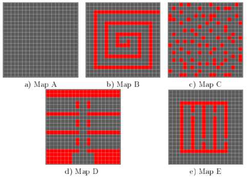
Fig.1. Topologies studied

The optimum theoretical values of idleness are calculated as follows: Let v the number of available cells of the environment. We consider that each agent visits one cell at each iteration. An agent thus visits the whole environment in v iterations. When the agent finishes its work, the most formerly visited cell will have an idleness of v - 1 (since the idleness of the current cell is equal to 0). For n agents, the optimal maximum idleness therefore worth (v/n) - 1. Optimal instantaneous average idleness is therefore: ((v/n) - 1) / 2.

At the end of these simulations, we hope to obtain idleness results substantially close to the theoretical optimum. Thus, we particularly expect from our simulations that the average idleness obtained on each of these 5 environments is substantially close to the theoretical optimal value.

• 4.2.    Non-obstacle environment (Map A)

Fig.2 shows the performance obtained with 8 sensors in a 20x20 cells environment containing no obstacles. Initially, the sensors are randomly located on the environment. This plot represents the average idleness and the worst idleness. It results that the average idleness is almost stable and very close to the theoretical optimum. However, for the worst idleness, it is not the same thing. The curve of the worst idleness does not converge towards stability and remains well above the optimum. Thus, with 8 sensors in a Non-obstacle topology, average idleness converges towards optimum, ensuring a good patrol.

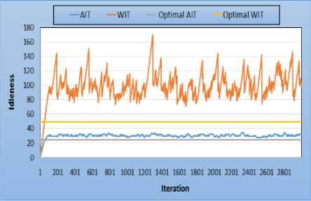
Fig.2. Non-obstacle topology - 8 sensors

Fig.3 shows the overall idleness for a variable number of sensors. For the average idleness like the worst idleness, when the number of sensors doubles, performance improve is observed. For the average idleness, we notice that whatever the number of agents, the values obtained are very close to the theoretical optimum value. However, for the worst idleness values are not as close to the optimal.

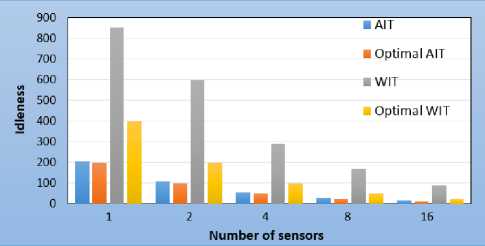
Fig.3. Non-obstacle topology - overall idleness

In this first environment, we can observe that the average idleness obtained by PreFap has almost reached a stability and is almost close to the theoretical optimal. This allows us to affirm that on this environment PreFap succeeds in carrying out a regular patrol.

• 4.3.    Spiral environment (Map B)

Fig.4 presents the values of average and worst idleness obtained with 2 sensors in a spiral environment. Initially, the sensors are randomly located on the environment. It results that the average and worst idleness fluctuate until a stability. This stability is the result of a perfectly regular visit of accessible cells of the environment. So, the patrol in a spiral environment is optimal in average and maximum idleness for a small number of sensors (<8). In fact, when the number of sensors is high, the constant is lost.

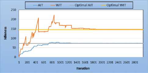
Fig.4. Spiral topology - 2 sensors

Fig.5 shows the performances of overall average idleness and overall worst idleness for a variable number of sensors. For the average idleness, we notice that when the number of sensors is small, that is less than 8, the overall average idleness is below the optimum value. In fact, for these cases, changes in idleness remain constant; sign of a perfectly regular visits from all accessible cells of the environment. For maximum idleness, we observe that the overall values for each number of sensors are not very far from the optimum value.

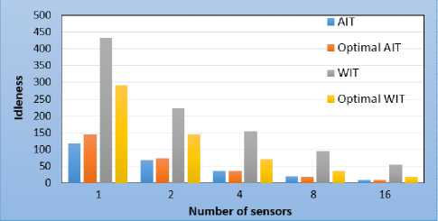
Fig.5. Spiral topology - overall idleness

The results of this second environment show that PreFap, in a spiral environment, succeeds squarely in reaching the theoretical optimal values both in terms of average idleness and maximum idleness. This means that monitoring has become perfectly regular.This regularity promotes rapid detection of various events that may occur during patrol.

• 4.4.    Environmentwith obstacle density (Map C)

Map C is a 20x20 cells environment containing 20% of randomly generated obstacles. This environment is an environment that has undergone a catastrophe because the obstacles are dispersed on either side of the environment. Fig.6 shows the performance with 8 sensors initially positioned randomly. It results that the average idleness is almost stable and very close to the optimum theoretical value. There is a quasi-constant of the curve of average idleness; But, that of maximum idleness, does not have a precise tendency.

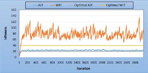
Fig.6. 20% obstacles topology - 8 sensors

Fig.7 presents the overall idleness obtained at the end of the simulations. It is seen in this plot that whatever the number of sensors, the overall average idleness is still close to the optimum theoretical value. However, the overall maximum idleness is very far. Thus, by increasing or decreasing the number of sensors, the trends observed in the Fig.6 remain the same.

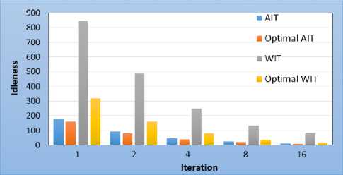
Fig.7. 20% obstacles topology - overall idleness

Like in this first environment, here we can observe that the average idleness obtained by PreFap has almost reached a stability. So, also on this environment,PreFap succeeds in carrying out a regular patrol.

• 4.5.    Corridor-rooms environment (Map D)

We now explore the behavior of PREFAP model on a complex environment consisting of several rooms to visit. In this case, these corridors and rooms. Fig.8 shows the average and worst idleness performance for the case of a single sensor on the Map D. The sensors always begin their exploration at the entrance of the hall. We note that, for a monosensor patrolling, the environment managed to be perfectly visited on a regular basis. Hence the constant changing environmental idleness.

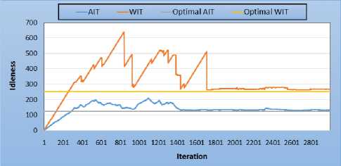
Fig.8. Corridor-rooms topology - 1 sensor

Overall idleness obtained at the end of the simulations are shown in Fig.9. The average idleness is still very close to the optimal. Note that in the case of 2 sensors, the overall average idleness is below the optimal. However, the overall maximum idleness is far from the optimal because of the great growth of the worst idleness at the beginning of the patrol

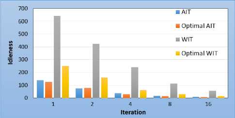
Fig.9. Corridor-rooms topology - overall idleness

One more time, PreFapsucceeds squarely in reaching the theoretical optimal values both in terms of average idleness and maximum idleness. So, monitoring has become almost regular.

• 4.6.    Imbricated rooms environment (Map E)

5.    Interpretations 5.1.    Exploration and patrol

Map E is another complex environment consisting of four interlocking pieces. Fig.10 shows the performance with 4 sensors initially positioned at the same place. As usual, the average idleness is almost stable and very close to the optimal. And the tendency of the worst idleness is similar to Non-obstacles topology and 20% obstacles topology.

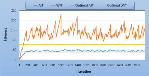
Fig.10. Imbricated rooms topology - 4 sensors

Fig.11 presents the overall average and maximum idleness obtained at the end of each simulation. As usual, we notice a close proximity between the overall average idleness and optimal average idleness. On the other hand, the overall maximum idleness is not as close to the optimal.

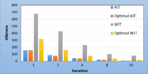
Fig.11. Imbricated rooms topology - overall idleness

Simulations of these environments have brought out two operating modes. Initially, the system is in a stage of exploration of the environment, then it changes to a more stable and efficient behavior. This stability behavior is due to some self-organization of the system through the marking of the environment. When the number of sensors is low, a stabilization of idleness values is observed on the spirals and corridors environments. Moreover, on the other topologies, this two-phase system is particularly at medium idleness.

• 5.2.    Advantages and shortcomings of PREFAP model

If we look at the average idleness, PREFAP is an effective solution for all topologies. In this case, we have shown that the proposed approach is sufficient to guarantee a low average idleness and very close to the theoretical optimum; including spiral and corridors environments. Sometimes the overall average idleness is below the optimal.

On the other hand, if we look at the maximum or worst idleness PREFAP gives results not very close to the optimum value. In addition, the maximum idleness is not stabilized; except for spiral corridors and environments when the number of sensors is low. Indeed, in these cases PREFAP reached the optimal.

More generally, one of the surprises of the PREFAP model is the obtaining of good performances, even optimal, in the case of the patrol with only one sensor. Indeed, we notice that average idleness decreases linearly with the number of sensors and allows to be more efficient on complex environments such as nested parts environments. Also, these performances show that environmental marking process can be a good solution for mono-agent problems.

Glad et al in [16], performed a comparative study between the EVAP and CLiNG models using the same environment topologies. By comparing the results of this study as presented in [16] with our results, we realize the relevance of the PREFAP model.

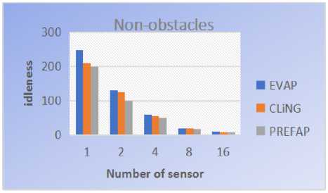
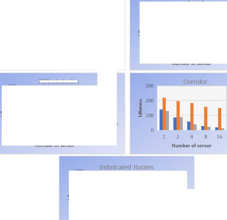
Like we can see on this Fig.12, on all the 5 environments used, PREFAP gave better results than EVAP and CLiNGin terms of average idleness. But in terms of maximum idleness, CLiNGwas better than PREFAP on the environment 20% of obstacles, like we can see on Fig.13. Because on this environment, Cling gave values of idleness much more minimal.

20% obstac es

■ EVAP

■ CLiNG

■ PREFAP

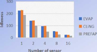
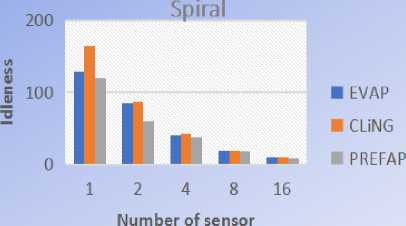
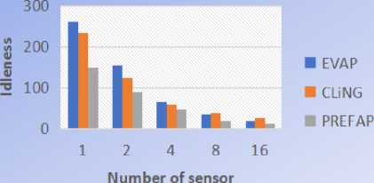
Fig.12. Comparison of the average idleness of EVAP, CLING and PREFAP on the 5 topologies studied

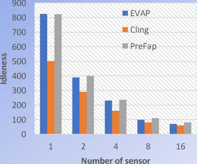
Fig.13. Comparison of the maximum idleness of EVAP, CLING and PREFAP on the 20% obstaclestopology

However, on all other topologies, PREFAP seems to provide more optimal results. This allows us to validate both the relevance and the satisfaction of our approach.

6.    Conclusion

In this article, we are interested in solving the problem of multi-sensor patrol in unknown environments; The patrol is a task that aims to minimize the time required to visit all accessible places in the environment.

A formulation of the multi-agent patrolling problem in unknown environments was presented as found in the literature. We presented the evaluation criteria to measure performance of a patrol strategy. The existing resolution’s approaches of the multi-agent patrolling problem in unknown environments have been described. From this state of the art, we proposed a hybrid approach of resolution with three components: a perception-reaction module for simple navigation, a strength-based module for obstacle avoidance and a module learning for decision making, particularly to come out of the deadlock. The perception-reaction module is used by sensors when no obstacle is perceived in their environment. In the event of obstacle detection, the force module is activated to allow the sensors to avoid collisions with obstacles in their environment. As we have shown, this force module can cause the sensor to be trapped in an area. To remedy this blockage, the sensor will use reinforcement learning.

We simulated our PreFap algorithm on 5 different environments with a population of 1, 2, 4, 8 and 16 sensors over a period of 3,000 iterations, evaluating the criteria of average idleness and maximum idleness. It can be seen that PreFap achieves very good performance in minimizing average idleness even when patrolling with a single sensor for each environment. But the worst idleness was not optimal for all environments precisely on 20% obstacles topology.

PREFAP is an effective patrol approach in environments with or without obstacles. Its character of regular patrol and minimization of idleness makes it possible to speed up the detection of events in environments. This approach can be used in applications to search for survivors following a disaster, to monitor the borders of an area, or to monitor a forest for the prevention of bush fires.

We plan to continue this work by integrating the results of our approach by varying a greater number of parameters, in particular the size of the environment, the number of iterations. One of the possible prospects in the short and medium term concerns the validation of our approach using a real physical network of mobile wireless sensors. These experiments would indeed collect valuable information on the effectiveness of our approach on real sensors; and to give an overview of his strengths and weaknesses.