A low cost indoor positioning system using computer vision

Published Online April 2019 in MECS DOI: 10.5815/ijigsp.2019.04.02

In the last decade, localization has become a substantial task for a wide range of applications. The evolution of the Global Positioning System (GPS) has been significantly swift since the introduction of the first GPS full operational capacity in 1995. Thus, its performance turns out to be stellar in outdoor environments. Otherwise, the system is restricted to accuracy within 1 to 10 meters. Due to this accuracy limitations, a new set of challenges have been created, one of them is the ability to increase the positioning accuracy to reach the centimeters scale. Therefore, Indoor Positioning System (IPS) is introduced to cope with the accuracy constrains including signal scattering and loss caused by the walls in an indoor medium. Lately, as a result of the gap between the prelude of GPS and IPS, indoor positioning turns into an active research and development subject in different fields.

The IPS market has a market estimation growth to 4.4$ billion by the year 2019, based on MarketsandMarkets, with a high requests in the field of logistics, health care, Localization Based Services (LBS) and transportation. “Strategy Analytics” reported that nowadays more than 80-90% of the daily time of the people is spent in an indoor environment. “IndoorAtlas” [9] in 2016 conducted a survey of the organizations desire to implement IPS at their sites, the survey has been asked to 301 respondents, the results declared that 72% of the organization have implement IPS or in the process of implementing it.

The raise of indoor localization evoked the demonstration of LBS in indoor environment which can boost the business market. Several technologies have been implemented in IPS caused the expansion of using it in many modern applications. These technologies are dependent on a set of parameters, and it is important to match these parameters with the application requirements [1]. Major challenges are confronting the versatility of an IPS, the accuracy of measuring the position of an object stays the major challenge. The mass market is still waiting for an optimal solution, which can revolutionize the business industry. However, there will be diversity in the system interpretation caused by various critical factors in an indoor environment. The challenges include: Non-line-of-sight (NLOS) cases where a radio signal transmission path are partially or completely obscured by obstacles, intense multipath caused by signal reflection from indoor barriers, temporary change in the movements of the medium, signal loss and scattering due to greater obstacles densities, high accuracy and precision request, variable lightning conditions and occlusion situations.[2]

Since locating objects and people has become a remarkable application in the modern life, the necessity of IPS increased in the market. A glimpse of IPS various applications will be enumerated. Furthermore, the applications diversity can be increased in the future by improving the performance of the system [2]. Applications include: Home entertainment; smart systems for lost objects detection and human motion gesture capturing system [3]. Location based services; Billing, searching services and providing a topological information on (cinemas, malls, museums, etc). Hospitals; Tracking patients in emergency cases and robotic assistant surgeries. Industry; robotic guidance [4] and robotic cooperation [5]. Transportation; Vehicles positioning inside parking garages [6] and synchronization of location information between the driver's mobile position and its car [7]. Logistics; Optimizing inventory tracking in warehouse systems and cargo management systems in airports.

The current paper discusses the development of a low cost optical-based IPS compared to the other technologies used. The total cost of the system is under 100$, which is considered cheaper to other vision systems that can exceed 500$. This promotes an indoor environment independent system, where the camera is already deployed in the scene. This situation can be ideal in warehouse locations. The software is compatible with different camera data buses including USB 2.0, USB 3.0, Camera Link, GigE Vision, IEEE 1394, achieving a high accuracy and precision results of the system within the range of 1 cm. The outcome values of the accuracy are based on the calibration of the Logitech C920 commercial camera. The development of tracking software that can track objects properly in real time operation in an indoor environment is proposed. The system is tested on the CUSBOT platform, which includes three agents with different RGB colors. The algorithm can deal with dynamic illumination of the scene which can affect the image with noise. The design and implementation of software for intercommunication between the CUSBOT agents, and the IPS work using MQTT protocol is deployed. The communication between the clients is useful for managing and transferring the data of the current system.

• II.    Related Work

  Based on camera vision system, in 2010, “Kohoutek

et al.” [23] proposed a novel indoor positioning method based on two main components, a spatio ‐ semantic interior building modeled in CityGML at a level of details

4 (LoD 4). “Boochs et al.” [24] in 2010, aimed to improve the positioning accuracy of an industrial robot to reach 0.05 mm. The setup was a test measurement cell where the robot is placed and the multi-camera system was mounted. “Chen and Lee” [25] in 2011, used only one fixed omnidirectional camera mounted on the ceiling of the room. The CCD camera operates at 15 frames per second with a resolution of 1280x960 pixels. AmigoBot robot platform was used with marker for positioning purpose and path planning mission. The vision algorithm detected the robot, targets and obstacles. “Huang et al.” [26] in 2012, developed a mobile robot localization system using ceiling landmarks by capturing the images using an RGB-D camera. In 2016, “Shim and Cho” [27] suggested a new vision-based technique for mobile robot localization by deploying two camera on the ceiling in an indoor environment. The dual camera configuration helped to reduce the complexity of occlusion situations, while maintaining an accurate localization.

• III.    Experimental Setting

  The proposed IPS work is designed in the control laboratory of Aerospace Engineering Department at Cairo University campus. It is an indoor environment independent system where an optical-based technology is used. A low cost commercial camera has been used for the proposed computer vision system, a Logitech C920, had an estimated price of 60$, was the best choice for such a low cost optical-based indoor positioning system. The camera has a complementary metal oxide semiconductor (CMOS) image sensor. It can reach a resolution of 2304 x 1536 with a frame rate of 2 fps. The resolution used for the current system is 1280 x 720 with a frame rate of 30 fps and RGB24 pixel format.

• A.    Perspective calibration

A spatial calibration is the pre-process of referring the acquired image pixels to real characteristics in the digital image. It can be used for accurate measurements in real-world units instead of pixel units, other usages are for camera perspective correction and lens distortion. Mapping is the process of relating each pixel to a real world location, a conversion ratio must be known between pixels and real world measurements; for example, 1 pixel equals 1 centimeter so a measurements of 5 pixels equals 5 centimeters.

Perspective calibration is used when the camera is mounted in an angular condition from the scene. It applies a linear correction based on the geometry of the scene. It is also called “Point coordinates calibration” which corrects camera angle distortion (perspective distortion) based on known distances between points. Lens distortion is not considered in this type of calibration. The proposed work is implemented in a way where the camera is mounted in an angular position from the working scene, so that a points coordinates calibration is required. Image coordinates are represented in pixels and the origin point of the image (0,0) is located at the top left corner while a world coordinates are represented in real-world units, like centimeters, and its origin point is located at an arbitrary location. The testing scene is located in the control laboratory (3rd floor) of the aerospace engineering department building, at Cairo University. The working scene in the room is highlighted with a scotch tape on the ground, an area of 391.5 cm x 549.5 cm (width x length) is specified for testing the proposed IPS. The view is captured from the camera which is mounted at height of 280 cm with a resolution of 1280 x 720 pixels at a frame rate of 30 fps.

As shown in Figure 1, the origin point is considered as (0,0,0) and located at the bottom left corner in the working scene. The z dimension is constant at 13 cm, which is the height of the rover that will be used later for the positioning task. So that, the origin point will be (0,0,13). Therefore, the z dimension is negligible while converting from pixels to real-world measurements. At a height of 13 cm, the x and y axes are divided to an equally 30 cm partitions in the working scene. 34 points are defined in the program, which are measured previously in the working scene. These are reference points in pixel coordinates used for calibration. Each point is corresponded in the real world coordinates to its match in the pixel coordinates.

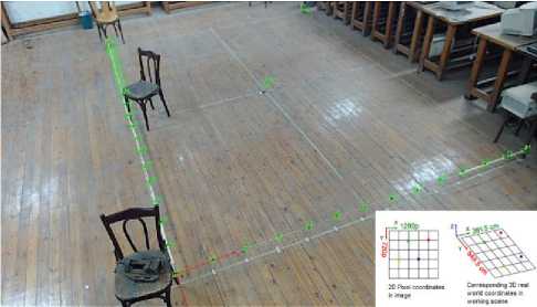
Fig.1. Points coordinates calibration

After implementing points coordinates calibration, as shown in Figure 1, the corrected image is displayed in Figure 2. The difference before and after the calibration is that each pixel in the acquired image is remapped to its new and corrected location. Based on the correction map in the calibration, the resolution is converted from 1280 x 720 to 1418 x 1443. So that, the angular view of the camera, from the working scene, has been corrected and the perspective distortion issue is solved. The correction is not applied to the live image acquisition; because it is a very slow process. However, it is used as a single reference image for converting pixels to real-world coordinates in real time.

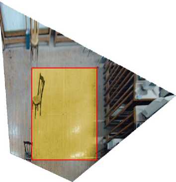
Fig.2.Corrected image

• B.    Calibration accuracy results

The combined error map is a 2D array containing the predicted position error for each pixel in the entire image. The generated map is an estimation of the positional error expected after the conversion of pixel coordinates to real-world coordinates. The error value indicates the radial distance from the real-world position. The positional error estimation of the real-world coordinates is equal, to or smaller than, the error value 95% of the time, which is called the confidence interval. [28]

The map has three main colors; black, shades of blue and white, as shown in Figure 3. The black and the dark shades of blue are indications of pixel coordinates with smaller errors, which mean a high accuracy of the real-world coordinate estimation for a pixel. The white and the light shades of blue are indication of a pixel coordinates with larger errors, which means a low accuracy of the real-world coordinate estimation for a pixel. The working scene fall in a high accuracy area of the map as it must be rigorous for the proposed IPS. The calibration accuracy results show a mean error and maximum error of 0.659 cm and 1.148 cm respectively, as depicted in Figure 4.

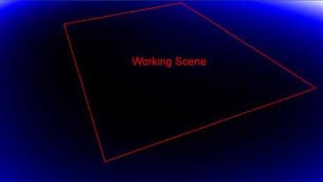
Fig.3. Calibration accuracy displayed in a combined error map

Calibration Accuracy

Display

Mean Error:

Max Error:

Std Dev:

% Distortion:

0.659445     centimeter

1.14832      centimeter

0.0627475    centimeter

0.576801

Error Range (centimeter)

Fig.4.Combined error map calibration accuracy results

Each pixel coordinate in the map has its error value e ( _i, j) , which refers to the largest possible displacement error for the estimated real-world coordinate (x,y) as compared to the real-world location (x true ,y true ). The following equation describes the error value calculation:

e ( i , j ) = 7 ⁽ x - x true ^{) 2} + ⁽ У - У rue ^{) 2          (1)}

• C.    Optimizing lighting conditions

The working scene, in the suggested IPS work, is subjected to two different sources of lightning; the sunlight shining directly through the room windows and several fluorescent lamp strip light attached in the ceiling of the room. Both sources are negatively affecting the image quality, especially that the room’s floor has some form of reflectibility, as shown in Figure 5.a. As a result, a tremendous information and features extraction from the image will be missed, causing an increased complexity and time consuming in the image processing. To overcome these issues, a blackout curtains are hung above the windows to prevent the sunlight penetrating the

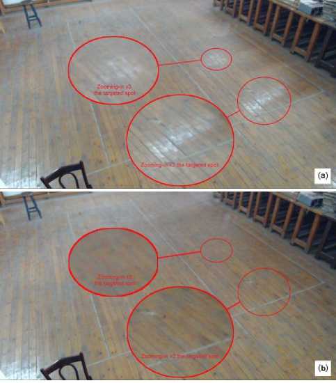
Fig.5.Working scene before and after correcting the lightning conditions as shown in (a) and (b) respectively room and a large paper sheets are attached to fluorescent lamp frames. The sheets are taking U shape to guarantee a maximum light scattering among the room before hitting the floor. Figure 5.b clarifies the scene after optimizing lightning conditions.

• IV.    Image Processing and Segmentation

Background subtraction method, image segmentation and processing are discussed. An RGB color planes extraction is performed, before any image processing, to optimize the color identification of the rovers. All these procedures in this section are applied to enhance the image before any tracking operation. The proposed IPS is tested on the CUSBOT platform, which is a robotic platform for multi-agent decentralized network. The multi-agent network is implemented by three rovers. Each rover is marked with one of the RGB colors for identification purposes. RGB color planes extraction is primary step.

• A.    RGB color planes extraction

Figure 6 shows the acquired image from the camera. The three rovers are covered with color markers for each color. A black cover hides the internal components of the rovers, which enhances the main rover color. Therefore, it can easily differentiate the pixel values of the colors. The 32-bit RGB image is represented for the three color planes with a bit depth of 2n, where n is the number of bits used to encode the pixel value. The 8-bit architecture is the depth bit used, so it can differentiate 256 different values ranging from 0 to 255. The RGB color space is represented by a color range from black (0,0,0) to white (255,255,255).

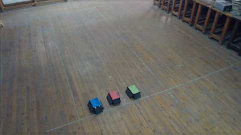
Fig.6. 32-bit RGB image acquired from the camera

The three 8-bit RGB color plane images, extracted from the raw 32-bit image, are illustrated in Figure 7. For the three color planes, it is evident that each rover with its unique color marker is identified within its relevant color plane. As a result, the highest pixel values are always related to the color marker of the rover. Furthermore, another aspect of the image analysis can be represented by a 3D view, as shown in Figure 8, in which the image is displayed using an isotropic view. Each pixel from the image source is demonstrated as a column of pixels in the 3D view and pixel value corresponds to the altitude. The light intensity is displayed in a 3D coordinate system.

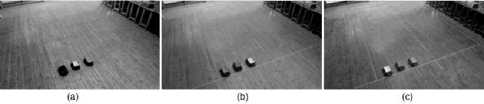
Fig.7. 8-bit images of red, green and blue extracted planes as shown in (a), (b) and (c) respectively

All the three extracted RGB planes are being analyzed with a 3D view. The resultant is a well-defined peak with the highest pixel values located at the color marker of each rover and identified in its relevant color plane. There are other peaks observed in the produced 3D map. However, they are not related to the object. These peaks correspond to the background scene, which will be subtracted later by background subtraction manipulation.

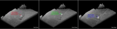
Fig.8. 3D view representation of the three 8-bit images of RGB planes extraction

• B.    Background subtraction

The proposed work is primary subjected to illumination changes in the scene and adapted to variable geometry in the scene. The fundamental idea of the algorithm is that the first image frame is stored as the reference frame image I_r and the current frame image I_c is being constantly subtracted from the pre-stored reference frame image I r . Afterwards, the image is segmented by thresholding to create a binary image. It is based on a criterion to ensure a successful and neat achievement of motion detection. Figure 9 shows the flow diagram of the proposed background subtraction algorithm. While Figure 10 shows the resultant binary images of the foreground mask, after thresholding the subtracted images, for the three RGB planes. These images detect the color marker of the rovers only for precise tracking. The subtracted background image B (x,y,t) is updated frequently by B (x,y,t+i), where i ∈ {0,..,n+1} and i is the delay value of the timer used until updating the next background reference frame. In order to, guarantee a reliable motion detection.

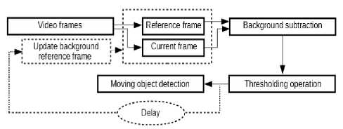
Fig.9. Flow diagram of the proposed background subtraction algorithm

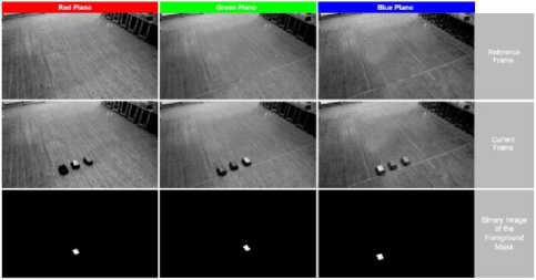
Fig.10. Binary images of the foreground mask after thresholding the subtracted images for the three RGB planes

A binary image is created where active pixels containing the motion information possess the value of “255” and non-active ones containing the background information possess the value of “0”. The following equation describes the approach:

B ( x , y , t ) = I c_c ( x , y , t ) - I r ( x , y , t )| >  Th (2)

Where:

B (x,y,t): subtracted background image which is the binary image of the foreground mask.

Ic (x,y,t): current frame image at time t.

I r (x,y,t): pre-stored reference frame image at time t.

Th: specified criteria for the threshold value.

• C.    Automatic thresholding

A histogram analysis is applied on the color marker of each rover in its relevant plane, after background

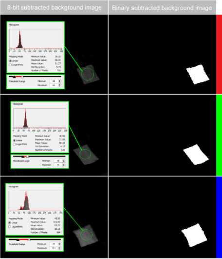
Fig.11. Adjusting threshold interval parameters based on histogram analysis to produce binary subtracted images for the three RGB planes subtraction approach, to identify the minimum and the maximum pixel intensity values in the 8-bit image. Therefore, the threshold interval parameters kmin and kmax can be determined based on these values. Figure 11 shows the adjustment of threshold interval parameters based on histogram analysis, to produce binary subtracted images for the three RGB planes.

Due to the illumination changes in the indoor scene over time; the pixels intensity values, which correspond to the color markers, vary frequently. Therefore, adjusting threshold interval through constant interval values is not efficient over time, as shown in Figure 11. In order to cope with this variation in values, a conversion of the 8-bit subtracted background image of the relevant planes to 2D pixels values array is needed, as depicted in Figure 12.

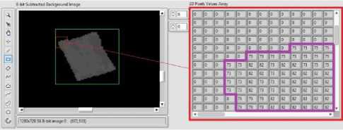
Fig.12. Analyzing the conversion of 8-bit subtracted background image to 2D pixels values array

The conversion is required to analyze the resultant 2D array and identify the pixel values that belong to the color marker. In Figure 12, the conversion from 8-bit image to 2D pixel values array target the color marker of the rover via Region of Interest (ROI). The 2D array created, represents the full ROI “green rectangle”, but the displayed values are for the smaller red rectangle. The “zero” values correspond to the background and the values inside the purple region match the color marker. Both values change slightly over time. The automatic update of the threshold interval is performed by continuously extracting the maximum value from the 2D array, which will be the input of the upper value of threshold interval. A constant value is subtracted continuously from the maximum value to create the input of the lower value of the threshold interval.

• D.    Advanced morphological transformation

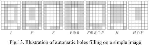
An Automatic holes filling is a morphological reconstruction operation, where binary morphological reconstruction is a morphological transformation that includes two images and the structuring element. Instead of a single image and structuring element exist in basic morphological transformation. The two images are the marker of the input image, where it is the beginning point of the transformation. In addition to the mask, which puts some constrains on the transformation. Figure 11 illustrates the process of automatic holes filling on a simple image.

Where:

• I:    binary input image I(x,y).

Ic: mask image, which is the complement of binary input image I(x,y).

• F:    marker image F(x,y). If (x,y) is on the border of I(x,y), then F(x,y) = 1-I(x,y). Otherwise, F(x,y) = 0.

• B:    structuring element used with defined pixels connectivity.

• H:    binary morphological reconstructed image with all holes automatically filled where H = [ R Ic (F) ]^c.

(a)                                    (b)

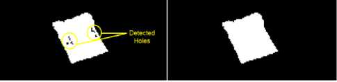
Fig.14. (a) Binary image with detected holes defect on the color marker (b) Binary morphological reconstruction of the image using automatic holes filling

For the working indoor scene, filling holes function in particles might be useful in tracking the color marker of the rovers in binary images. There are cases where the color marker of the rovers is not properly thresholded from the grayscale images. The reason behind this defect is that while the color markers are moving along the working scene area, they are being captured and observed from different angles with respect to the camera. This leads to different intensity values of the color marker pixels. This variation in pixels intensity can be misleading in thresholding the color marker. As a result, holes can be created as particles corresponding to the background and set as “0” in the binary images, as depicted in Figure 14.a. While Figure 14.b shows the binary morphological reconstruction of the image using automatic holes filing.

• V. Proposed Tracking Methods and Localization Results

The camera is deployed in the room at a height of 280 cm from the ground. The working area scene for testing purposes is 549.5 cm x 391.5 cm. It is mounted in an angular condition from the scene. Therefore, point coordinates calibration is applied to correct the perspective distortion based on 34 checkpoints. The calibration accuracy results reported a maximum error of 1.14 cm, a minimum error of 0.60 cm and a mean error of 0.65 cm. Blackout curtains are utilized for isolating the indoor scene from external illumination along the day to reduce the noise in the image processing.

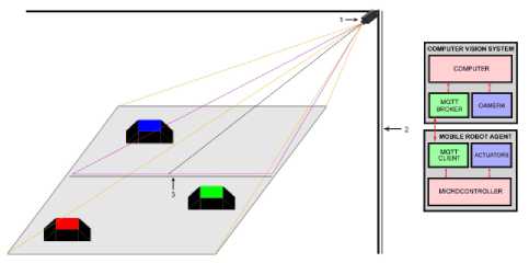
Fig.15. Proposed camera deployment in real indoor environment and IPS vision based architecture

The proposed IPS has been tested on a robotic platform for multi-agent decentralized network called “CUSBOT”, where the positioning data of the vision system are sent to the controller of the rovers throughout MQTT. The positioning data is used for group formation among decentralized agents “rovers”. Several formations are tested in this work including: line, rendez-vous and triangle formations. The tests are evaluated using centroid approach for localization. An illustration of the imaging system in a real indoor environment and the system architecture are elaborated in Figure 15. Figure 16 represents the general block diagram of the proposed IPS.

Where:

X = Pixel coordinates of X in the image.

Y = Pixel coordinates of Y in the image.

Pixel values = Numerical value of each pixel.

Pixel values are always equal to “1” or “0” due to working on binary images. After thresholding operation, the background value is always equal to “0” and the object, to be tracked, is always equivalent to “1”. This means that any (x or y) pixel related to the background will be eliminated from equation 4.1 and 4.2; because its pixel value will be “0”. Centroid approach on binary images is better than grayscale images, because of the exemption of pixels related to background. While on grayscale images both pixel corresponding to the background and object are considered.

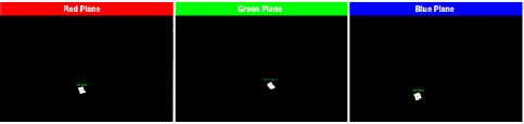
Fig.17. Centroid approach localization in binary images of the three RGB planes

Figure 17 shows the centroid approach localization in binary images of the three RGB planes. Experimental results are demonstrated in Table I, the accuracy reported is within 1 cm as depicted before in Figure 3. The centroid approach localization is applied after thresholding process in Figure 10.

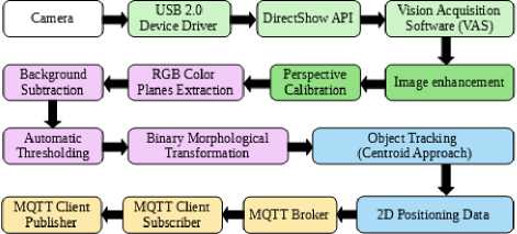
Fig.16. General block diagram of the proposed IPS

Table 1. Experimental localization results of centroid approach

	x (pixels)	y (pixels)	x (cm)	y (cm)
Red Rover	605.20	505.27	81.50	32.47
Green Rover	711.29	475.34	126.31	30.01
Blue Rover	504.39	546.48	39.36	28.43

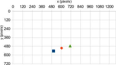
After applying “Points coordinates” calibration as shown in Figure 1, the centroid pixel coordinates of three rovers extracted from the three RGB planes is illustrated

A. Centroid approach

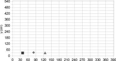
in Figure 18. The calibrated centroid real-world coordinates of the three rovers is illustrated in Figure 19.

Centroid approach computes the center of energy of an image. It is calculated by the following standard centroid equation for the (x,y) values of the centroid:

x (pixels)

0  120 240 360 480 600 720 840 960 1080 1200

x

^ ( X ) х Pixel Values ^ Pixel Values

У =

^ (Y ) х Pixel Values ^ Pixel Values

Red Rover

Green

Rover

Blue Rover

Fig.18. Centroid pixel coordinates of the three rovers

0  30  60  90 120 150 180 210 240 270 300 330 360 390

x (cm)

Fig.19. Calibrated centroid real-world coordinates of the three rovers

• B.    Particle measurements approach

Particle measurements approach is used to analyze and measure particles in a binary image. These particles are characterized by several parameters: areas, lengths, coordinates, axes, shape features, etc. Particle measurements method is classified as a point tracking approach in object tracking. Moving objects are expressed by their features or parameters while tracking. Thresholding is a pre-process phase for particle measurements and analysis.

Particle area identification is calculated based on several factors:

• •    Number of pixels: The area of a particle excluding the holes in it. The unit is expressed in pixels.

• •    Particle area: The area of a particle excluding the holes in it after applying spatial calibration and correcting the image. The unit is expressed in real-world measurements.

• •    Scanned area: The area of the full acquired image. The unit is expressed in real-world measurements.

• •    Ratio: The ratio of the particle area to the scanned area. It is expressed in the following equation:

  Ratio =

  
  

Particle Area

Scanned Area

• •    Number of holes: The amount of holes inside a particle in an image.

• •    Area of holes: Total area of the holes inside a particle.

• •    Total area: The sum of the particle area and the area of the holes.

Figure 20 shows the particle analysis of area for the three RGB rovers in its relevant plane. The rovers have been magnified four times for a better display and inspection. The green boxes are called “Bounding Rectangle”, which targets the localization of the rovers. Bounding rectangles are identified based on two parameters: center of mass (x,y) of the particle and first pixel (x,y) of the particle.

Red Rover

Green Rover

Blue Rover

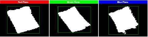
Fig.20. Particle analysis of area for the three RGB rovers in its relevant plane

The results of an experimental particle analysis of area, for the three RGB rovers in its relevant plane, are depicted in Table II. Total area of the rovers is an important parameter to identify the criteria of the maximum and minimum pixels, while the rovers are moving across different perspective and angles from the camera. A hole has been detected in the blue rover; because automatic holes filling were disabled in the blue plane. In order to illustrate the performance in different planes with automatic holes filling activated and deactivated.

Table 2. Experimental particle analysis of area results for the three RGB rovers in its relevant plane

	Red Rover		Green Rover		Blue Rover
	pixels	cm2	pixels	cm2	pixels	cm2
Particle Area	1652	354.96	1554	365.82	1895	358.37
Area of Holes	0	0	0	0	1	0.173
Total Area	1652	354.9	1554	365.8	1896	358.5
Convex Hull Area	1733	389.88	1634	407.26	2123	419.29
Image Area	921600	586750	921600	586750	921600	58675 0
% Particle Area/Image Area	0.17925 %	0.0605 %	0.1686 %	0.0623 %	0.2056 %	0.0610 %
% Particle Area/Total Area	100%	100%	100%	100%	99.94%	99.95 %

Unlike the centroid approach, which computes the centroid of the entire binary image including its full particles, particle’s center of mass calculates the center of mass of each particle independently in the entire binary image. In this proposed work, the rovers in its relevant planes are the targeted particles to be tracked. The rovers are being represented as a one solid particle that has a specific area. Particle’s center of mass is related to the pixel coordinates of the image. The coordinates are being represented with respect to the origin point of the image (0,0) and located at the top left corner. The center of mass of a particle (Pi) is equal to its center of gravity (G), composed by a number of (N) pixels.

A general formulation to compute the center of gravity (G) is expressed in equation 6. Equations 7 and 8 represent the average destination of the central points of the horizontal and vertical segments within a particle respectively.

G =

i = N

E Pi i=1

Red Rover

Blue Rover

Green

Rover

Fig.22. Center of mass M x and M y pixel coordinates of the three rovers

G x

i = N

E Xi i=1

i = N

E Y

G y

i = 1

Red Rover

Green Rover

Blue Rover x (cm)

Fig.23. Calibrated center of mass Mx and My of the three rovers in real-world coordinates

Derived equations 9 and 10 are expressed, for a specific form of particle’s center of mass. The equations represent the center of mass X,Y respectively. Each particle in the entire image has a different area so that the center of mass X,Y is computed independently.

M x = 1( E X )            (9)

M y = 4( E ^Yi )            (10)

yAi

Figure 21 shows the particle measurements approach localization in binary images of the three RGB planes. Experimental results are demonstrated in Table III, the accuracy reported is within 1 cm as depicted before in Figure 3. Particle measurements approach localization is applied after thresholding process in Figure 10.

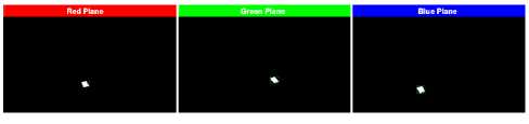
Fig.21. Particle measurements approach localization in binary images of the three RGB planes

Center of mass (Mx) and (My) is retrieved from equations 9 and 10 respectively. While the total area A of the particle used in these equations are extracted from Table II.

The results of particle’s center of mass, for localization of the three rovers, are similar to the centroid approach. Figure 22 shows the center of mass (Mx) and (My) pixel coordinates of the three rovers. After applying “Point Coordinates” calibration, as shown in Figure 1, the calibrated center of mass (Mx) and (My) is illustrated in Figure 23 in real-world coordinates for the three rovers.

C. Mean shift method

Mean shift algorithm is commonly used nowadays in object tracking applications. Some of the mean shift algorithm usages are: Object tracking, image segmentation, clustering, pattern recognition, filtering, and information fusion.

For object tracking purposes, the desired object to be tracked must be characterized by a feature space. The most common feature space used is the color histogram; due to its robust representation of the object appearance.

These results in describing the moving objects are by their histograms. The histogram feature based target representation is adjusted by spatial masking, including an isotropic kernel.

The mean shift algorithm is an approach for detecting the location of a local mode, which is the local maximum of a kernel-based estimate of a probability density function. Histogram extraction, derivation of new position and weight computation are the settings required to perform an object tracking for an image frame.

For a non-parametric mean shift method, the algorithm mode determines the density function according to the distribution of points. This approach of object tracking localizes the targeted object for a long time and effectively compared to other tracking approaches.

The general framework of the proposed mean shift algorithm is introduced in Figure 24. There are three main stages for mean shift tracking methods, as depicted in Figure 25. Firstly, target modeling, where the desired object to be tracked, is identified in the present frame of the image throughout an ROI. The targeted model is represented based on color histogram feature space with an isotropic kernel. Secondly, mean shift convergence

occurs in the subsequent frame of the image, where a searching process begins with the current histogram and spatial data retrieved from the previous frame to find the best target match candidate by maximization of the similarity function. While the centroid of the object is moving from the current destination to a new one, the kernel is also moving until the convergence of the similarity function is satisfied.

Therefore, the targeted object location is updated. Thirdly, model and location update where the targeted model and its location are updated based on blending parameters.

Table 3. Experimental localization results of particle measurements approach

	Red Rover		Green Rover		Blue Rover
	pixels	cm	pixels	cm	pixels	cm
Center of Mass M x	605.1271	81.5876	711.1094	126.4128	504.3895	39.4188
Center of Mass M y	505.2421	32.6239	475.8442	30.0111	546.4285	28.4831
First Pixel X	609	87.7189	711	132.9501	510	45.4671
First Pixel Y	482	43.8273	451	43.0763	519	40.9263
Bounding Rectangle Left	578	73.2974	682	118.1269	474	30.1605
Bounding Rectangle Top	482	45.2128	451	43.4427	519	41.2658
Bounding Rectangle Right	634	90.4882	743	135.3506	534	48.1781
Bounding Rectangle Bottom	530	20.6452	500	17.1838	577	13.6659
Bounding Rectangle Width	56	17.1907	61	17.2236	60	18.0176
Bounding Rectangle Height	48	24.5676	49	26.2589	58	27.5998
Bounding Rectangle Diagonal	73.7563	29.9848	78.2432	31.4036	83.4505	32.9604

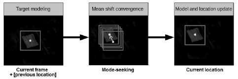
Fig.25. Main stages of mean shift method

1) Target modeling

At a current frame, an ROI must be drawn around the targeted object to be tracked. Afterwards, retrieving the data points and computes the approximate location of the mean of this data. For the proposed work, the mean shift method is dealing with 8-bit grayscale images for each RGB plans independently. Therefore, the target model has a probability distribution of monochrome histogram.

Equation 11 describes the probability (q) of color (u), where u=1,…,m in target model.

n qu = CE k (I lx<-II 2)^[ b (xi - u)]        (ii)

i = 1

C = [ E k (II x i ll )] ^-1               (12)

i = 1

Where:

C: normalization constant.

xi: [i=1,…,n] indicates the pixels locations of target model at centroid y0.

b(xi): indication of color bin of the color at xi.

δ: kronecker delta function such as:

5 ( d ) =

1 if d = 0

0 otherwise

Where:

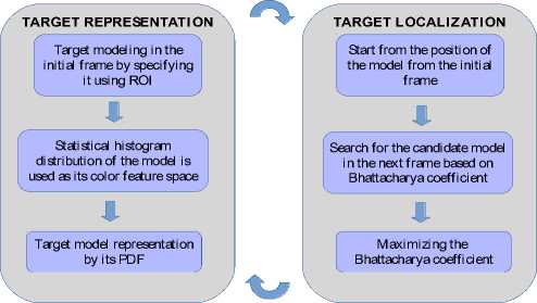
Fig.24. General framework of the proposed mean shift algorithm

k(||x||2) tends to qu if b(xi) = u.

• k: kernel profile weights contribution to the center of the target model.

kernel K is a function of ||x||2:

K ( x ) = k ( x ²)              (14)

Properties of kernel profile k:

• •    k is non-negative.

• •    k is non-increasing.

• •    k is continuously piece-wise.

  Equation 15 describes the probability (p) of the color (u) in the target candidate, where y_i, i=1…,n_h indicates the pixel locations of the target candidate at its centroid (y).

  
  

  w_i

  
  

  m

  = ∑ δ [ b ( y_i - u )]

  u = 1

  
  
  
  
  
  
  

  p_u

  
  

  n_h C h ∑ k ( i = 1

  
  

  y - y_i h

  
  

  )δ [ b ( y_i ) - u ]

  
  
  
  

  Where:

  C_h is the normalization constant.

  n

  C h = [ ∑ k ( x i II² )] ^{- 1}          (16)

  i = 1

  2) Mean shift convergence

  For mean shift convergence, a mean shift vector must be defined first to identify the direction from the centroid (y₀) at the current frame in the image to the new centroid (y₁) at the next frame where the highest density exists.

  To find the best target candidate in the next frame from the current frame, a maximization of the similarity function represented in the bhattacharya coefficient should take place. The likelihood maximization depends on maximizing the weight function (w_i) of the window of the pixels in tracking window.

  Bhattacharya coefficient (ρ) in equation 17 is used to compute the similarity and measurements between the target model (q) and the target candidate (p) by its color (u) at its location y, as shown:

  
  

  For a minimization in the distance between two distributions, it requires maximization in bhattacharya coefficient. The maximization in bhattacharya coefficient can be reached by maximizing the second term in equation 18. The maximization in bhattacharya coefficient is dependent on maximizing the weight function w_i in equation 19. The weight is recomputed in every iteration.

  3) Model and location update

  For updating the model and location of the target, the object’s centroid moves from the current position y to a new position (y₁) in the next frame. To describe the new model and location of the object, mean shift iterative equation is used.

  n_h

  ∑ x_iw_ig_i

  y 1 = ^{i =} _n ¹ _h                       (20)

  ∑ w_ig_i

  i = 1

  
  

  ρ ( p ( y ), q ) = ∑ _u ^m ₌₁ V p_u ( y ) q_u      (17)

  Where:

  • •    ρ i s the c os ine of vectors ( √ p 1 ^{, ... ,} √ p m )^T and ( √ q 1 ^{, ... ,} √ q m )^T. Increased value of (ρ) indicates a well color matching.

  • •    y indicates the location of the target model at the current frame with its color probability (p).

  • •    z indicates the estimation of the new target model location at the next frame near its previous location (y), where its color probability does not change remarkably.

  Equation 18 describes the bhattacharya coefficient of candidate target p(z).

  
  

  ρ ( p ( z ), q ) = ¹ ∑ _u ^m _{= 1}   p_u ( y ) q_u

  
  

  n_h + ^Ch ∑ w i k ( 2 i = 1

  
  

  z - y_i h

  
  

  )

  
  
  
  

  Where:

  w_i is the weight function in the following equation 19:

  
  

  VI. Results and Discussion

  The evaluation of the proposed IPS work has been tested through “Formation Control”. The purpose of this test is to achieve three types of formation: line, rendezvous and triangular formations, based on the positioning data of the IPS, using centroid approach. Both the robots and the IPS are connected to the same router network. MQTT protocol is used for the communication between the positioning data from the IPS to the wifi module ESP8266 installed on the rovers’ boards.

  To be able to perform a formation test, each robot of the CUSBOT platform must be informed by its current position in the working scene and its neighbor’s robots current position in real time. This process is implemented in the system through MQTT protocol, the positioning data are extracted by the centroid approach for object tracking and then the values are shared to a MQTT publisher.

  Figure 26 provides the architectural design of the communication between IPS positioning data and clients subscribers through MQTT protocol. The output data of the IPS is a 2D real-world coordinates of the targeted object. The data is shared to an implemented MQTT client publisher where Eclipse Mosquitto is the broker that regulates the data traffic between the publisher and the subscriber.

  
  

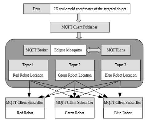
Fig.26. The architectural design of the communication between IPS positioning data and MQTT client subscribers

There are three topics used by the broker in this work, each topic is relevant to a position of a specific robot such as: Topic 1, 2 and 3 that contains the current positioning data of the red, green, blue robots respectively. These topics, including the values, can be seen through a MQTT utility extension in Google Chrome called “MQTTLens”.

Each robot is considered as a MQTT subscriber, so that the red, green, and blue agents are subscribed to their relevant topic 1, 2, and 3 respectively. They are subscribed additionally to the other topics also so they can be notified by their own current position and their neighbors’ current positions also to be able to perform the desired formation. Each robot is considered as a MQTT subscriber, so that red, green, blue agents are subscribed to their relevant topic 1, 2, and 3 respectively. In addition to the subscription to the other topics; they can be notified by their own current position and their neighbors’ current positions, to be able to perform the desired formation.

The positioning data values are updated simultaneously with minimal delay of 50 ms, as an update rate for real time application. Whenever the values are updated by the centroid approach for object tracking, the MQTT topics are also updated by the new values for each robot. Therefore, the three agents are notified by their new positioning values and their neighbors’ new positioning values too.

• A.    Line formation test

A primary formation test is performed to achieve a vertical line formation by the robots. At first, the robots are dispersed in a random way in the working scene, and then they are able to communicate with each others to fulfill the required formation.

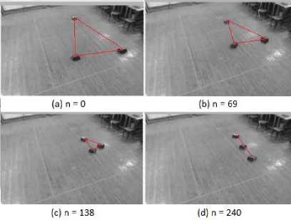
Fig.27. Development of vertical line formation using MQTT protocol between the proposed IPS and CUSBOT platform

Figure 27 illustrates the development of vertical line formation using MQTT protocol between the proposed IPS and CUSBOT platform, where n is the number of frames acquired by the optical system. At first, the robots are randomly placed in the working scene, as shown in Figure 27.a. At the end, after acquiring 240 frames, the rovers accomplished their mission by achieving a vertical line formation as seen in Figure 27.d.

Figure 28 shows the 2D real-world coordinates map of CUSBOT agents achieving vertical line formation using MQTT protocol. The yellow bar in the graph illustrates the threshold of accuracy for the vertical line formation of the robots. The experimental results reveal that the agents are not perfectly aligned in a vertical line. The displacement of each centroid of the rovers is below the range of 10 cm, which is an acceptable tolerance.

The paths of the agents, from their starting locations to their ending locations until they reach the desired formation, are dependent on the CUSBOT platform performance. While the positioning data sent to the agents through MQTT protocol, do not provoke any lags in the performance of the agents.

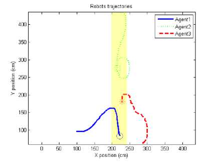
Fig.28. 2D real-world coordinates map of CUSBOT agents achieving vertical line formation using MQTT protocol

• B.    Rendez-vous formation test

Another formation test is performed to achieve a rendez-vous formation by the robots. At first, the robots are dispersed in a random way in the working scene, and then they are able to communicate with each others to acquire the desired formation. The final target of the rendez-vous formation is that each rover should be to the nearest distance between its own centroid and its neighbor’s one.

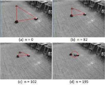
Fig.29. Development of rendez-vous formation using MQTT protocol between the proposed IPS and CUSBOT platform

The development of formation using MQTT protocol between the proposed IPS and CUSBOT platform is demonstrated in Figure 29. At the initial frame, where n=0, the agents are scattered in the map randomly, as seen in Figure 29.a. Then, the robots began to move closer to each others to achieve the rendez-vous formation at frames n=82 and n=102 respectively which is illustrated in Figure 29.b and Figure 29.c. The rovers accomplished their rendez-vous formation at frame n=195, as depicted in Figure 29.d.

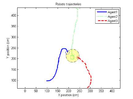
Fig.30. 2D real-world coordinates map of CUSBOT agents achieving rendez-vous formation using MQTT protocol

Figure 30 shows the 2D real-world coordinates map of CUSBOT agents achieving rendez-vous formation using MQTT protocol. The yellow spot in the graph illustrates the rendez-vous zone, where the centroids of the rovers are at the nearest area from each others. The experimental results show that the diameter of the zone, where the agents end their trajectories is in the range of 50 cm, which is an acceptable tolerance. The paths of the agents, from their starting locations to their ending locations until they reach the desired formation, are dependent on the CUSBOT platform performance. While the positioning data sent to the agents through MQTT protocol do not provoke any lags in the performance of the agents.

• C.    Triangular formation test

A third formation test is performed to achieve a triangular formation by the agents. At the beginning the agents are placed randomly in the working scene, and then they are able to communicate with each others to acquire the desired formation. The final target of the triangular formation is that the three rovers compose a shape of triangle with a three sides equally. The distance of the equal sides between the centroid of each agent is predetermined by the CUSBOT platform.

Figure 31 illustrates the development of triangular formation using MQTT protocol between the proposed IPS and CUSBOT platform. At the beginning, at the initial frame n=0, the agents are placed at random distances from each others, as seen in Figure 31.a. Then, they start to regroup each others to form a triangle formation with equal sides, as depicted in Figure 31.b and Figure 31.c. After acquiring a number of frames n=42 and n=98 respectively. At last, the agents achieve the final triangular formation, as seen Figure 31.d, where n=150 frames.

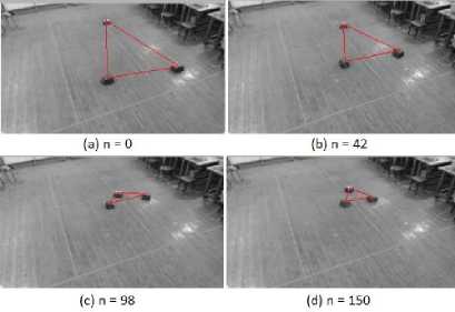
Fig.31. Development of triangular formation using MQTT protocol between the proposed IPS and CUSBOT platform

Figure 32 demonstrates the 2D real-world coordinates map of CUSBOT agents achieving triangular formation using MQTT protocol. The yellow area in the graph represents the final triangular formation achieved by the agents, where each centroid of the rovers is distributed equally from its neighbors to form the three sides of the triangle. The experimental results reveal a measurement of 100 cm for each side of the triangle. This value is already determined by the agents’ formation algorithm.

• D.    Other tests

Several object tracking approaches are tested based on the proposed IPS work. The methods include: particle measurements and mean shift. The experimental results are induced from circular and linear trajectory tests, where both (X,Y) real-world coordinates graph and (X,Y) positions versus time graph are illustrated.

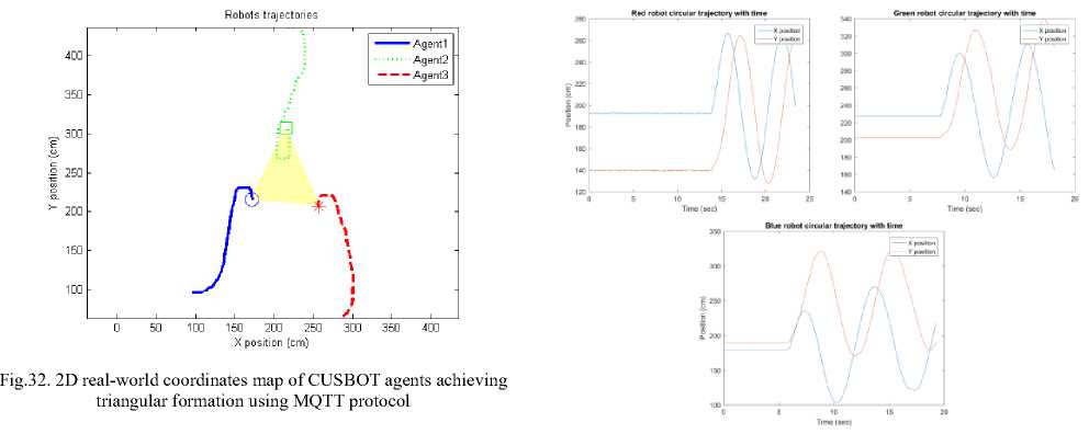
Fig.34. X-Y Circular trajectory positions of the RGB agents with time based on particle measurements approach

• 1)    Circular trajectory test

Figure 33 illustrates the circular trajectory tracking of the RGB agents based on particle measurement approach. Each rover is identified and tracked in its relevant RGB plane. The average circular trajectory is 1.5 to 2 cycles. The experimental results show consistency in tracking and neat trajectory.

Figure 34 depicted the X-Y Circular trajectory positions of the RGB agents with time based on particle measurements approach. The experimental results show clean sinusoidal waves of the X-Y positions with respect to time. The straight line in the graphs indicates that the rovers are in a stationary state, while the sinusoidal waves represent the movements of the rovers in a non-stationary state.

Figure 35 illustrates the circular trajectory tracking of the RGB agents based on mean shift approach. Each rover is identified and tracked in its relevant RGB plane. The average circular trajectory is 2 to 2.5 cycles. The experimental results show consistency in tracking and neat trajectory.

Figure 36 demonstrates the X-Y Circular trajectory positions of the RGB agents with time based on mean shift approach. The experimental results show clean sinusoidal waves of the X-Y positions with respect to time. The straight line in the graphs indicates that the rovers are in a stationary state, while the sinusoidal waves represent the movements of the rovers in a non-stationary state.

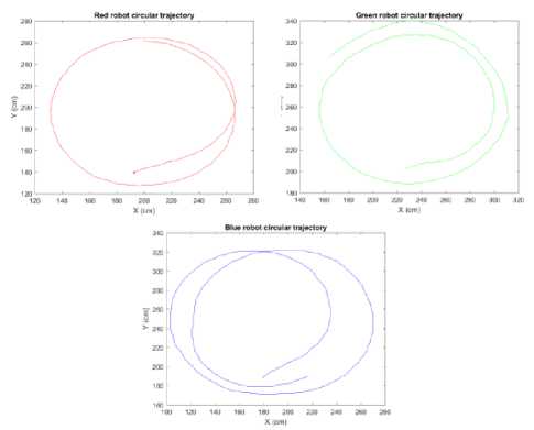
Fig.33. Circular trajectory tracking of the RGB agents based on particle measurements approach

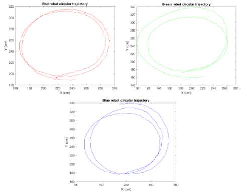
Fig.35. Circular trajectory tracking of the RGB agents based on mean shift approach

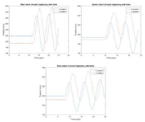
Fig.36. X-Y Circular trajectory positions of the RGB agents with time based on mean shift approach

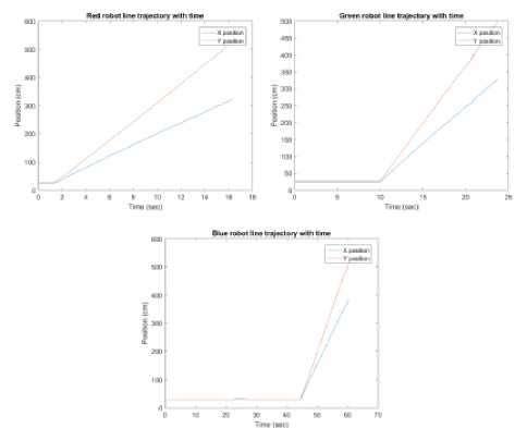
Fig.38. X-Y Linear trajectory positions of the RGB agents with time based on mean shift approach

• 2)    Linear trajectory test

Another type of trajectory tests is performed, besides the circular trajectory tracking. A linear trajectory tracking is tested, where the movement of the rovers is in diagonal shape along the working scene. Each rover is identified and tracked in its relevant RGB plane.

Figure 37 demonstrates the linear trajectory tracking of the RGB agents based on mean shift approach. The starting point of the agents is set near the (0,0) position in the working scene, while the ending point is set near the furthest point in the map which is (391.5,549.5). The experimental results show consistency in tracking and neat linear trajectory.

Figure 38 illustrates the X-Y linear trajectory positions of the RGB agents with time based on mean shift approach. The graphs show both overlapped lines and separated lines. The overlapped lines indicate the agents in a stationary state, while the separated lines prove the agents in a non-stationary state.

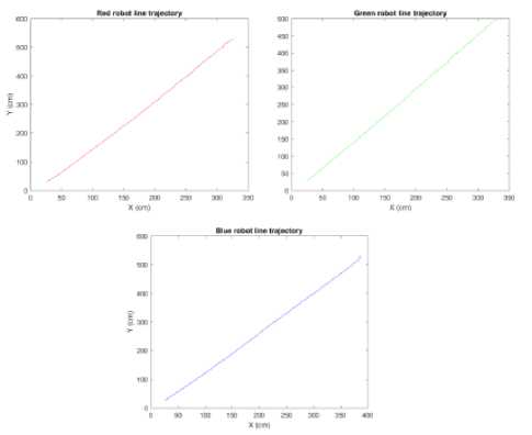
Fig.37. Linear trajectory tracking of the RGB agents based on mean shift approach

• E.    System benchmark

To evaluate the performance of the proposed work, there are several key parameters that affect the system performance. Thus, a system benchmark is executed to obtain a performance assessment. The IPS in this research is tested to track robots for multi-agent decentralized network, which is a real-time application. For that reason, a requirement of fast system response should be available to prevent any lag in the system performance during any phase of the object tracking and the MQTT communication that can affect the attitude of the rovers.

Table 4. Selected parameters for system performance assessment

Parameter	Average Execution Time
Reference frame	51.4 ms
Current frame	31.8 ms
Image subtraction	1.1 ms
RGB color planes extraction	2.7 ms
Image calibration	91.2 ms
Thresholding	0.1 ms
P.M.O – Erosion	2.9 ms
A.M.O – Automatic holes filling	3.3 ms
Display	2.3 ms

Table IV shows the selected parameters for system performance assessment, where various metrics have been chosen for the evaluation. The average execution time of the parameters is computed based on 30 inspection runs. Reference frame, current frame and image subtraction are operations related to image acquisition and background subtraction. The image calibration parameter recorded the highest average execution time. However in the proposed work, the image calibration is done once before the software starts. In other words, it is not executed in each iteration and frame continuously. RGB color planes extraction, thresholding, erosion and automatic holes filling are processes related to image segmentation and processing.

A brief comparison between the three object tracking approaches used in the proposed work is demonstrated in Table V.

Table 5. Brief comparison between the three object tracking approaches used in the proposed work

	Centroid	Particle Measurements	Mean shift
Scanning area	Entire image	Entire image and based on selected metrics	Selected ROI
Image type	Binary	Binary	8-bit
Effect of noise	Affected	Controllable	Unaffected
Tests performed	Formation missions (Linear, rendezvous and triangular)	Circular trajectory	Circular and linear trajectories
Tracking accuracy	Moderate	High	Highest
Detected spikes in tracking results	Detected	Undetected	Undetected
Tracking results filtration	Needed	Unwanted	Unwanted
Paths intersection situation	Passed	Passed	Passed

• VII. Conclusion and Future Work

The proposed work was targeted to develop a low cost optical based IPS, using a Logitech C920 commercial camera. The system was tested on the CUSBOT platform agents and shows promising results for object tracking using computer vision. The proposed work is summarized as following:

Tweaking the camera attributes so it can provide a resolution of 1280 x 720 pixels with a frame rate of 30 fps and a video format of RGB24. For that reason, these attributes are sufficient for the proposed IPS providing unremarkable lags or delays.

The BCG values of the raw image for a proper image enhancement are adjusted. Therefore, the final result is a richer colors image, which provides more obvious objects and details.

Applying a perspective calibration algorithm “Points Coordinates Calibration” to the camera, which is mounted in an angular condition from the scene, corrects the angular distortion of the camera. In addition, high accuracy results are achieved in localization within the range of 1 cm.

An indoor working scene environment located in the control laboratory of the aerospace engineering department, at Cairo University campus, was chosen to test the proposed IPS.

RGB color planes extraction is applied to the raw 32-bit image to identify each agent of the CUSBOT platform with its unique color marker within its relevant color plane. As a result, the intersection trajectories problem of the CUSBOT agents in the map is solved.

Background subtraction technique is implemented to separate the foreground from the background by generating a foreground mask, where a binary image is created containing the pixels corresponding to the moving objects in the scene. The reference frame is updated periodically to deal with the illumination change of the indoor scene over time.

Thresholding is used as an image segmentation technique to produce the binary images of the RGB planes based on specific threshold interval. An automatic update of the threshold interval algorithm is developed to cope with the variation of the pixel values in the color markers.

Advanced morphological transformation, in form of automatic holes filling by binary morphological reconstruction, is used to the binary images to fill any detected holes in the color markers at any location in the map.

Implementing intercommunication software using MQTT protocol, for sending the positioning data, is utilized. The positioning data are sent to each CUSBOT agent to perform formation tests.

Several formation tests were executed, including: line, rendez-vous and triangular formations, based on the centroid approach. Other object tracking approaches are used, such as: particle measurements and mean shift methods. These approaches are introduced in circular and linear trajectory tests.

The test results were accurate with an acceptable tolerance range. According to the three object tracking results, the mean shift method gives the highest tracking accuracy comparing to the centroid and the particle measurements approaches.

For future work, multiple cameras can be introduced to the system to expand the coverage of the working scene to include multiple rooms or whole floor, rather than one room. Besides, they can be used to extract 3D information and positioning data from the image as a stereoscopic vision system. The system can also be improved to operate in both indoor and outdoor environments. In addition, several navigation algorithms can be implemented for path planning and obstacle avoidance purposes.