A machine learning algorithm for biomedical images compression using orthogonal transforms

Biomedical image compression is an extremely important part of modern computing. By having the ability to compress images from their original size, the required storage space in computer memory space of images can be reduced. In addition, the transmission becomes easier and less time-consuming. In fact, the problem is the very large amount of data contained in a medical image can quickly saturate conventional systems [1]. There exist two types of compression: lossless compression where reconstruction data is identical to the original; and lossy compression where there is a loss of data. However, lossless compression is limited because compression rates are very low [2]. The compression ratio of the lossy compression scheme is very high. Lossy compression algorithms are generally based on orthogonal processes, such as the discrete cosine transform [3-6], the discrete Walsh transform [3], the

Karhunen-Loeve transform [3, 5, 7], the discrete wavelet transform [1, 2, 4, 5, 8, 9] and the Discrete Chebyshev Transform (DChT) [10-13]. All these transforms are unitary, symmetrical, reversible and the energy of the image before and after processing remains unchanged. However, although these compression methods can have a good image quality of restoration with high compression rates, they are slow in terms of coding time and do not produce a good compromise between the Peak Signal to Noise Ratio (PSNR) and the compression ratio (CR). To overcome this drawback, vector quantization (VQ) and Machine Learning (ML) algorithms are most often associated to increase the performance. VQ techniques have been widely used in the area of image coding because of their ability to achieve a low bit rate [14-19]. VQ techniques achieve a low bit rate by exploiting the correlation and redundancy between blocks [20, 21]. VQ breaks the transformed image to be compressed into vectors which are quantized to the closest codeword. VQ is achieved by only sorting or transmitting the address of the closest codeword, instead of the whole vector of image pixels [22]. To improve the VQ, a ML algorithm can be used to calculate the codebook. Also, K -Means algorithm is often used to calculate and generate the optimal codebook that can be adapted to the transformed image [23, 24]. Several papers have been published concerning image compression using the orthogonal transform and some analytical solutions are described in [2-5]. Lu and Chang presented in [15] a snapshot of the recently developed schemes. The discussed schemes include mean distance ordered partial codebook search (MPS), enhance LBG (Linde, Buzo and Gray) and some intelligent algorithms. In [12], Prattipati and al compare integer Cosine and Chebyshev transform for image compression using variable quantization. The aims of their work were to examine cases where DChT could be an alternative compression transform to DCT. However, their work was limited to the grayscale image compression and further, the use of a scalar quantification does not allow them to reach a high PSNR. H. B. Kekre, P. Natu and T. Sarode presented in

• [19]    a fusion of Vector Quantization and Hybrid Wavelet Transform (HWT). They proposed a color image compression method based on two types of vector quantization: Kekre’s Median Codebook Generation (KMCG) and Kekre’s Fast Codebook Generation (KFCG). They obtained fewer errors than in the LBG algorithm and the image quality is better.

For biomedical images, all the information may be needed for diagnosis. Diagnosis based on the biomedical image cannot tolerate the distortion on the image. After the compression process, the reconstructed image should be identical to the original image. To achieve high rates, we focused on the two orthogonal transforms (Walsh and Chebyshev). We adapt these methods by an intelligent algorithm for high compression rate and no loss of data. Our method minimizes the distortions on the reconstructed images. Further, we observed that when the image is transformed with DWaT or DChT, and the codebook is calculated with a learning algorithm, the compression has very good parameters.

The rest of the paper is as below. Section 2 briefs on the concept of discrete Walsh transform, discrete Chebyshev transform and describes both vector quantization and Huffman encoding. Section 3 includes the results and the performance analysis. The implementation issues and comparisons are performed. Section 4 concludes the work.

• II.    Materials And Methods

In this session, we describe the set of methods used to develop our compression algorithm. In our proposed algorithm, we use a Machine Learning algorithm. K -Means clustering is an unsupervised learning algorithm that helps us with the Split method to construct our codebook necessary for vector quantization step. Thus, in this session, we will describe the three main steps of our compression scheme. The Fig. 1 illustrates the block diagram of the proposed compression and decompression scheme.

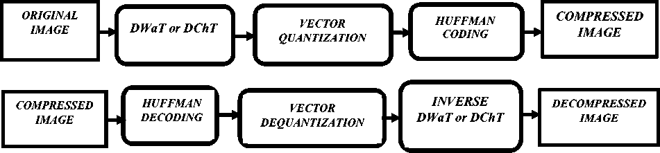
Fig.1. Block diagram of compression and decompression scheme.

The transformations refer to the conversion of the images from the time domain to other domains such as frequency domain through orthogonal bases. The image in the new domain brings out specific innate characteristics which can be suitable for some applications. In this work, we used Walsh transform and Chebyshev transform.

• A. Discrete chebyshev transform (dcht)

Chebyshev transform is obtained from the Chebyshev polynomials. The orthogonal Chebyshev polynomials are commonly used to analyze, approximate, synthesize, or reconstruct signals and images [25]. Discrete Chebyshev Transform (DChT) is an approach based on discrete Chebyshev polynomials. For a given positive integer N (the vector size) and a value n in the range [ 1, N-1 ], the N order orthogonal Chebyshev polynomials T_k ( x ) , k = 1,2,..., N - 1 are defined using the following recursive relation defined in [10-12, 26-28]:

T0 (x)     N,

T (0) = NEE I2EET (0),(2)

^{k (} ) N N + k    k - 1 ^{k - 1 (} )

Tk (1) = {1+k\ '/1 T (0) •

• 1 N

Tk (x) = Y1Tk (x — 1) + 7;Tk (x — 2) • k = 1,2,..., N—1, x = 2,3,...,1 ,(5)

Where

—k (k +1) —(2 x —1)( x — N — 1) — x at time index x. The inverse DChT is given in [27-29] by (9):

N —1

f ( x ) = Z F ( k T k ( x )             (9)

k =0

x = 0,1,2,..., N — 1

Now, let consider a function with two variables f ( x , y ) sampled on a square grid NxN points. Its DChT is given by (10), [12, 29-31]:

N — 1 N — 1

F ( j , k ) = Ц f ( x , y T ( y ) T k ( x )   (10)

x = 0 y = 0

j , k = 0,1,2,..., N — 1

And its inverse DChT is given by (19):

N — 1 N — 1

f ( x , y ) = ZZ F ( j , kT j ( y ) T k ( x )    ⁽¹¹⁾

j = 0 k = 0

• x , y = 0,1,2,..., N — 1

• B.    Discrete walsh transform (dwat)

Walsh functions are already discrete and thus easy to manipulate. The sequence of a Walsh function is determined as the number of zero-crossings per unit time interval.

The Walsh function W ( k , x ) is defined on the interval [0 1] in [32] by (12)

2 ^Y —1

W ( k , x ) = ^ W ( n /2 ^k ) win ( x 2 ^Y , n , n + 1 )    ⁽¹²⁾

n =0

where N = 2 ^k ;

x ( N — x )

_Y = ^{( x + 1 )( x —} N ^— 1 ) ²       x ( N — x )

for x e ( a , b ) for x £ [ a , b ]

for x e { a , b }

The forward DChT of order N is defined in [12, 27-29] by (8):

N I

F ( k ) = £ f ( xT k ( x )           (8)

x = 0

k = 0,1,2,..., N — 1

Where F (k) denotes the coefficient of orthonormal Chebyshev polynomials. f (x) is a one-dimension signal win represented the window function

When x = mJ N and for some integer 0 <  m <  N it comes that

W ( k , m/N ) = W k ( m/N ) 5 m , n = W_k ( nN ) 5 m , n = W_k ( m , k/N )

The orthonormality property of the Walsh functions is expressed by (14)

( W ( m , x ) , W ( n , x ) ) = 3 _m , n            ⁽¹⁴⁾

The discrete orthogonality of Walsh functions is defined in [32] by (15)

£ W ( m , NN ) W ( n , N N ) = N 3 _m , _n         (15)

i = 0

Consider a function f ( n ) defined in a discrete form on a compact, its Walsh transform is given in [32, 33] by (16)

N - 1

F ( m ) = ^ f ( n )W_t ( m , n )          (16)

n = 0

Where W ( m , n ) is a Walsh function of rank m, with m = 0,1,2,........., N - 1

The inverse DWaT is defined in [33] by (17):

1 N -1

f ⁽ n ) = T_r^ F ⁽ m ^)W k ⁽ m , n )         ⁽¹⁷⁾

N m = 0

Where with n=0, 1, 2, ..., N-1

For a function with two variables f ( n , m ) sampled on square grid N ² points, its 2D Walsh transform is given in [34] by (18)

N - 1 N - 1

F ( u , v ) = ^^ W_k ( u , v ) f ( n , m ) W k ( u , v )     ⁽¹8)

n = 0 n = 0

Where W ( u , v ) is the Walsh matrix having the same size as the function f ( n , m ) . The inverse 2D transform is also defined in [34] by (19)

1   N - 1 N - 1

f ( n , m ) = —2 ^^ W k ( n , m ) F ( u , v)W_k ( n , m ) (19) N n = 0 n = 0

Two techniques are used to perform the quantization of coefficients resulting from the discrete Walsh transform and discrete Chebyshev transforms, scalar quantization and vector quantization. If one refers to the theory of the distortion factor introduced by Shannon [2, 4], the best performance is always reached in theory with vectors instead of scalars. We have then adopted vector quantization of DWaT and DChT coefficients.

• C.    Vector quantization

• a.    Basic concepts

Vector quantization (VQ) was developed by Gersho and Gray [16, 17, 35]. A vector quantizer q may be defined in [36] by an application of a set E into a set F c E as (20).

E ^ F c E x =(x0,...,xk-1) ^ q(x) ^^

= x e A = { y_i , i = 1,..., M } , У, e F

A ˆ is a dictionary of size M and dimension k . E is partitioned by S = { S. , i = 1,..., M } , with s =J   ^x = y I .

¹   I q ⁽ x )      ¹

The distortion between x and x d ( Jx, x ) is a positive quantity or zero [18-21, 35-42] given by (21):

d ( ;c, x ) = || x - J f ||² = ]T ( X ( i ) - X ( i ) ) 2    (21)

i = 1

Where L is the vector size.

The total distortion of the quantizer for a given codebook is then:

1      LF (                              1

D ( q ) = | — I ^x ^ l Minimum d ( X, Yj ) I ⁽²²⁾

V L ) i =1 ^ Yj e Codebook    ^{X       7} J

The optimal quantizer ( q ) is that which minimizes the distortion for a random sequence of vectors X , where X has the probability p ( X ), it has to verify the condition D ( q * ) < D ( q ) . A and S determine entirely q and we can write :

D ( q ) = D ( A, S )

Where

D (. 4 , S ) = E ( d ( X , q ( X ) ) )

= £ P r ( x e S i ) J d ( x , yjx e S ) p ( x/x e S ) dx

Most of the classical vector quantization algorithms are based on two important properties [36, 43]:

-

-

If A ˆ is given, then the best partition of the input space is p (^ A ) , obtained by matching each X to vector y_t to A minimizing d ( x , x_} ) . This rule of nearest neighbor.

If S is given, then assume that for every S nonzero probability in a space k-Euclidean,

3 x ( S )/ E ( d ( X , x ( S ) )/ X e S )     (24)

= min E ( d ( X , u )/ X e S )

x ( S ) thus corresponds to a generalized centroid to S . Under these conditions, the best alphabet to reproduction is x ( S ) = { x ( S ) , i = 1,..., N } .

For the construction of our codebook, we used a machine learning algorithm that performs with unsupervised learning. Our unsupervised learning relies on the K -Means algorithm with the splitting method .

• b.    K-Means algorithm

The K-Means algorithm is at the basis of many standard methods of vector quantization [23]. Proceeding from M training vectors x(n), 1 ≤ n ≤ M, the problem is to split this set into K groups S i such that the optimal conditions are satisfied. The procedure of data classification is simple and easy for clustering [23, 44, 45]. K-Means is an algorithm leading to a local optimum satisfying the following conditions [46, 47]:

• a)    Choose K vectors Y_i(0) , initialize m, the index of iterations, to 0;

• b)    Classification: at iteration m, store the vectors {x(n), n= 1, ...., M} in the S i (m) by applying the

rule of the nearest neighbor from the vectors Y j (m);

• c)    Updating of code vectors   Y j (m  +  1)  =

centroid(S i (m)), 1 ≤ i ≤ K ;

• d)    End of the test on the gain in distortion compared to the previous iteration. If the result is negative, go to the step b.

It is obvious that in K -Means, we need all the training sequence for every iteration and the quantizer is not available as long as the procedure is not completed. Thus, the data must be part of the training sequence, and the groups change with each iteration. This is ideal for the case with medical images in which the images that represent data have to be used for the construction of codebooks. This is not the case of some method such as the most use in vector quantization Linde, Buzo and Gray (LBG) algorithm [15, 35, 48]. In the LBG algorithm, a part only of the input sequence is used to construct the quantizer, and, provided that the input sequence of vectors produced by the source is stationary and ergodic, the implementation remains practically optimal for any vector produced later. Since we are manipulating medical images, we chose for our compression scheme the K -Means algorithm instead of using a part of the input sequence to build the quantizer. We used all the input sequence in order to have a very low distortion. The algorithm of K -Means in our scheme is used with the splitting method. Vectors have the same probability and the entropy H increases.

• c.    Splitting Method

The Splitting operation serves to modify the initial codebook used by the K-Means algorithm. It is based on the probabilities of occurrence Pi of vectors of the codebook obtained during the first classification. A vector i of the codebook is then split if its probability Pi is high. Thus, the splitting of vectors of the codebook helps to balance the distribution of vectors of the training sequence during classification and thus, optimizes the partition of the codebook. Indeed, a splitting is successful if a class Si containing a Vi vector is split in two class Vi/2 vectors: one vector that has a great probability of occurrence is then replaced by two equiprobably vectors of lower probability of occurrence [49, 50].

VQ makes it possible to have a good quantification of the image during the compression. However the codebook generated during quantification is not always optimal, the reason why we introduced a training algorithm ( K -Means) to calculate the codebook. K -Means calculate and generate the optimal codebook that can be adapted to the transformed image [23]. K -Means does not solve the equiprobability problem between the vectors. Thus we coupled the K -Means with the Split method to have equiprobably vectors of lower probability of occurrence. This allows us to create a very suitable codebook for image compression and to be able to close the lossless compression techniques.

• D.    Huffman coding

  The Huffman coding is a compression algorithm based on the frequencies appearance of characters in an original document. Developed by David Huffman in 1952, the method relies on the principle of allocation of shorter codes for frequent values and longer codes to less frequent values [2, 4, 51-54]. This coding uses a table containing the appearance frequencies of each character to establish an optimal binary string representation. The procedure is decomposed into three parts:

• -    First, the creation of the frequencies appearance of the character table in the original data.

• -    Afterwards, the creation of a binary tree according to the previously calculated table.

• -    And lastly, encoding symbols in an optimal binary representation.

• E.    Performance evaluation

There are four parameters to evaluate the performance of our compression scheme: Mean Square Error (MSE), Maximum Absolute Error (MAE), Peak Signal to Noise Ratio (PSNR) and the Compression rate (CR). For an image represented by 256 grayscale ranging between 0 and 255. The MSE and PSNR are defined in [14, 21] as (25).

• 1     M - 1 N - 1

^MSE = 7777 SE ( I 0 (M) - I r (IJ) )   ⁽²⁵⁾

M N i = 0 j = 0

With I image as to compress and I reconstructed image and ( M, N) the size of the image. The PSNR is given by (26).

PSNR = 10 log₁₀ -55-          (26)

• ¹⁰ ( MSE J

  The MSE represents the mean error into energy. It indicates the energy of the difference between the original image and the reconstructed image. PSNR gives an objective measure of the distortion introduced by the compression. It is expressed in deciBels (dB). For a high PNSR and a low MSE, the decompressed image is closed to the original image.

  The Compression rate (CR) is defined as the ratio between the uncompressed size and compressed size. The CR is given in [2, 4, 55] by (27) and (28).

  
  

  MAE = max 1 1 ₀ ( i , j ) - I_r ( i , j )|        (29)

  
  

  CR =

  
  

  size of compressed image size of original image

  
  
  
  

  In percentage from the CR expression is given by (28)

  
  

  CR (%) = 100 -

  
  

  size of compressed image

  
  

  size of original image

  
  

  X 100

  
  
  
  

  Maximum Absolute Error (MAE) defined by (29) shows the worst-case error occurring in the compressed image [56].

  
  

  • III.    Results And Discussion

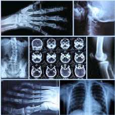
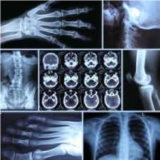
  In order to validate our proposed algorithm for biomedical images compression, we have performed an objective evaluation with the parameters presented in the previous session on test images from Fig.2. Thus, we present our obtained results with two utilized transforms: DWaT, DChT. The comparison between DWaT and DChT are made. We use our algorithms on the images of other articles finally to compare our algorithm with those of the literature. This in order to conclude on the effectiveness of our algorithms.

  • A. Results

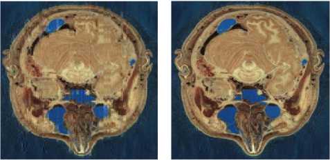
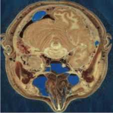
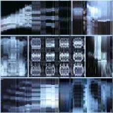
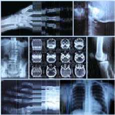
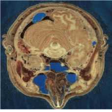
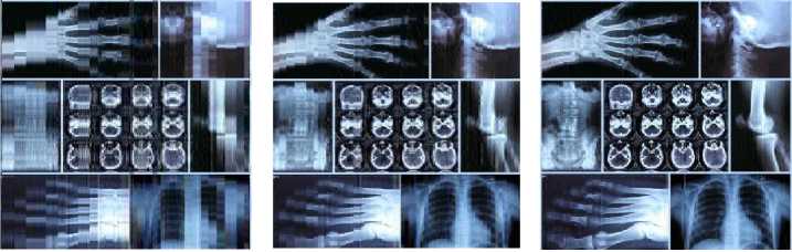
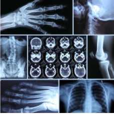
  MATLAB software was used to simulate our new image compression scheme. We use eight images from [57, 58] as test images to evaluate our scheme compression. These images represented in the fig. 2. Image size is 512 x 512 x 3 bytes.

  
  
  

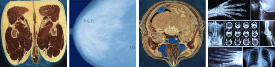
  (d) General- (I4)

  
  

  (a) Pelvis- (I1)

  (b) Mammography- (I2)

  (c) Head - (I3)

  

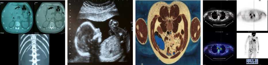
  (e) Fracture- (I5)

  (f) Echography- (I6)

  (g) Abdomen- (I7)

  (h) Strange Body- (I8)

  Fig.2. The test images [57, 58]

  
  

Table 1 presents the results obtained with DChT and table 2 those obtained with DWaT.

Table 1. Recapitulative of results with DChT Method

Images	Evaluation Parameters	Codebook Size
		64	128	256	512
Pelvis- (I1)	PSNR (dB)	20.85	24.38	33.35	Inf
	MSE	534.11	236.98	30.01	0
	MAE	7.78	4.94	1.76	0
	CR (%)	99.90	99.87	99.82	99.78
	CT (s)	175.81	172.57	175.44	201.64
	DT (s)	12055.1	10943.55	12654.48	12319.96
Mammography- (I2)	PSNR (dB)	34.55	40.64	50.46	Inf
	MSE	22.77	5.60	0.58	0
	MAE	1.41	0.72	0.18	0
	CR (%)	99.90	99.86	99.82	99.78
	CT (s)	180.65	175.76	178.53	191.56
	DT (s)	12698.6	11075.48	11111.27	11123.04
Head- (I3)	PSNR (dB)	23.14	26.82	37.05	Inf
	MSE	315.16	135.03	12.81	0
	MAE	5.98	3.67	1.19	0
	CR (%)	99.91	99.87	99.82	99.78
	CT (s)	173.69	169.75	178.62	198.76
	DT (s)	10746.27	11016.27	10705.48	11614.41
General- (I4)	PSNR (dB)	18.41	21.42	27.73	Inf
	MSE	936.89	468.14	109.54	0
	MAE	9.93	6.40	2.83	0
	CR (%)	99.89	99.86	99.82	99.78
	CT (s)	167.15	164.41	207.24	194.43
	DT (s)	11770.12	11528.36	10794.08	12188.45
Fracture- (I5)	PSNR (dB)	21.89	24.70	32.61	71.80
	MSE	419.87	220.33	35.60	0.004
	MAE	5.72	3.80	1.28	0.00008
	CR (%)	99.89	99.85	99.82	99.78
	CT (s)	164.62	165.10	184.36	241.83
	DT (s)	10468.87	10774.21	10762.52	11022.65
Echography- (I6)	PSNR (dB)	23.88	29.09	36.95	56.09
	MSE	265.75	80.01	13.11	0.15
	MAE	4.90	2.55	1.16	0.06
	CR (%)	99.87	99.82	99.76	99.70
	CT (s)	146.23	155.49	170.2	199.29
	DT (s)	8945.45	10076.84	10308.12	10767.65
Abdomen- (I7)	PSNR (dB)	21.11	24.91	33.28	Inf
	MSE	502.9	209.49	30.54	0
	MAE	7.30	4.47	1.80	0
	CR (%)	99.89	99.87	99.82	99.78
	CT (s)	160.2	168.71	218.65	276.15
	DT (s)	10301.2	10564.08	11187.09	11279.2
Strange Body- (I8)	PSNR (dB)	23.34	26.76	34.37	Inf
	MSE	301.13	137.10	23.73	0
	MAE	4.04	2.51	0.86	0
	CR (%)	99.90	99.87	99.82	99.78
	CT (s)	172.71	165.91	176.24	216.17
	DT (s)	12868.87	12390.25	12902.74	13011.2

Table 2. Recapitulative of results with DWaT Method

Images	Evaluation Parameters	Codebook Size
		64	128	256	512
Pelvis- (I1)	PSNR (dB)	21.05	24.28	31.15	Inf
	MSE	510.11	242.54	49.88	0
	MAE	7.70	5.08	2.42	0
	CR (%)	99.89	99.86	99.82	99.78
	CT (s)	6.93	9.89	16.06	34.27
	DT (s)	11.43	14.99	22.22	43.57
Mammography- (I2)	PSNR (dB)	35.33	41.35	50.01	Inf
	MSE	19.05	4.75	0.64	0
	MAE	1.31	0.68	0.21	0
	CR (%)	99.85	99.80	99.75	99.78
	CT (s)	4.95	5.99	9.59	32.09
	DT (s)	7.88	9.30	14.16	40.93
Head- (I3)	PSNR (dB)	23.06	26.33	33.52	Inf
	MSE	321.0	151.29	28.89	0
	MAE	6.07	4.02	1.76	0
	CR (%)	99.90	99.86	99.82	99.78
	CT (s)	7.08	9.54	16.72	36.52
	DT (s)	11.97	14.38	22.93	46.15
General- (I4)	PSNR (dB)	19.21	22.86	27.57	Inf
	MSE	780.1	336.2	113.8	0
	MAE	9.08	5.50	3.14	0
	CR (%)	99.89	99.85	99.81	99.78
	CT (s)	6.67	9.86	16.18	31.02
	DT (s)	11.38	14.76	22.72	42.91
Fracture- (I5)	PSNR (dB)	21.78	24.20	28.14	51.39
	MSE	430.67	246.85	99.6	0.47
	MAE	5.79	4.14	2.45	0.02
	CR (%)	99.88	99.85	99.81	99.78
	CT (s)	6.95	9.04	13.74	69.16
	DT (s)	11.50	13.97	19.84	78.01
Echography- (I6)	PSNR (dB)	23.89	28.73	36.95	50.38
	MSE	265.78	87.04	13.11	0.59
	MAE	4.95	2.70	1.16	0.19
	CR (%)	99.87	99.82	99.76	99.70
	CT (s)	5.29	7.70	12.15	23.98
	DT (s)	8.87	11.78	17.44	32.57
Abdomen- (I7)	PSNR (dB)	21.11	24.60	30.93	Inf
	MSE	502.9	225.3	52.45	0
	MAE	7.30	4.69	2.36	0
	CR (%)	99.89	99.86	99.82	99.78
	CT (s)	7.04	9.78	16.71	35.48
	DT (s)	11.48	14.77	22.53	44.58
Strange Body- (I8)	PSNR (dB)	23.40	26.03	31.80	52.06
	MSE	297.6	162.17	42.95	0.40
	MAE	3.79	2.55	1.79	0.02
	CR (%)	99.89	99.85	99.82	99.78
	CT (s)	7.62	11.16	15.35	72.45
	DT (s)	12.24	16.26	21.18	81.48

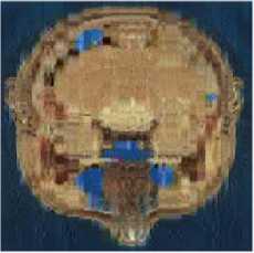
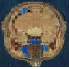
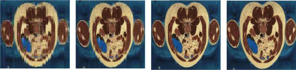
We can observe in Table.1 and in Table.2 the variation of PSNR, MSE, MAE, CR, CT (Compression Time) and DT (Decompression Time) according to codebook size. For a codebook size of 512, the values of PSNR are very high and they closer infinity for some images. The compression ratio ranges between 99.72% and 99.90% whatever the image and the codebook size. We can also notice that when the codebook size increases, the CR decreases slightly. Our results are then very satisfactory given the good compromise between PSNR and CR. The Fig. 3 and Fig. 4 present some of our test images decompressed using DChT and DWaT respectively. From these images, we confirm that the quantization step enormously influences the compression system especially as regards the choice of codebook size. For the same simulation with the same configurations, the settings such as PNSR, MSE and CR may be slightly different. This is because we assumed in our program during the learning phase, that if no vector is close to the codeword, we use a random vector by default. We can also see that the image quality is good when the codebook size is 256 or 512.

Codebook Size: 64

Head- (I3)

Codebook Size: 128

Codebook Size: 256

PNSR: 23.14dB; MAE: 5.98; PNSR: 26.82dB; MAE: 3.67; PNSR: 37.05dB; MAE: 1.19;

Codebook Size: 512

PNSR: Inf; MAE: 0;

MSE: 315.16; CR: 99.91%; MSE: 135.03; CR: 99.87%;    MSE: 12.81; CR: 99.82%;

Codebook Size: 64

General- (I4)

Codebook Size: 128

PNSR: 21.42dB; MAE: 6.40;

Codebook Size: 256

MSE: 0; CR: 99.78%;

Codebook Size: 512

PNSR: 18.41dB; MAE: 9.93;

PNSR: 27.73dB; MAE: 2.83;

PNSR: Inf; MAE: 0;

MSE: 936.89; CR: 99.89%;

MSE: 468.14; CR: 99.86%;

MSE: 109.54; CR: 99.82%;

MSE: 0; CR: 99.78%;

Abdomen- (I7)

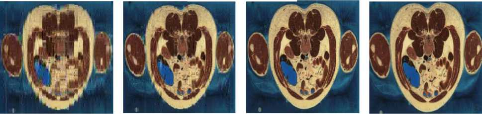
Codebook Size: 64

Codebook Size: 128

Codebook Size: 256

Codebook Size: 512

PNSR: 21.11dB; MAE: 7.30;

PNSR: 24.91dB; MAE: 4.47; PNSR: 33.28dB; MAE: 1.80;

PNSR: Inf; MAE: 0;

MSE: 502.9; CR: 99.89%;

MSE: 209.49; CR: 99.87%;

MSE: 30.54; CR: 99.82%;

MSE: 0; CR: 99.78%;

• Fig.3.    Head, General and abdomen images compressed and decompressed using DChT

  

  Codebook Size: 64

  PNSR: 23.06dB; MAE: 6.07;

  
  

  Head- (I3)

  

  Codebook Size: 128

  PNSR: 26.33dB; MAE: 4.02;

  
  
  

  Codebook Size: 256

  PNSR: 33.52dB; MAE: 1.76;

  
  
  

  Codebook Size: 512

  PNSR: Inf; MAE: 0;

  
  

  MSE: 321.0; CR: 99.90%;

  MSE: 151.29; CR: 99.86%;

  MSE: 28.89; CR: 99.82%;

  General- (I4)

  

  Codebook Size: 128

  Codebook Size: 64

  Codebook Size: 256

  PNSR: 27.57dB; MAE: 2.83;

  PNSR: 19.21dB; MAE: 9.09; PNSR: 22.86dB; MAE: 5.50;

  
  

  MSE: 0; CR: 99.78%;

  

  Codebook Size: 512

  PNSR: Inf; MAE: 0;

  
  

  MSE: 336.2; CR: 99.85%;

  MSE: 780.1; CR: 99.89%;

  MSE: 109.54; CR: 99.82%;

  MSE: 0; CR: 99.78%;

  Abdomen- (I7)

  

  ^{Codebook Size: 64           Codebook Size: 128}           Codebook Size: 256          Codebook Size: 512

  PNSR: 21.11dB; MAE: 7.30;  PNSR: 24.91dB; MAE: 4.47;    _{PNSR: 33.28dB; MAE: 1.80;  PNSR: Inf; MAE: 0;}

  
  

MSE: 502.9; CR: 99.89%;    MSE: 209.49; CR: 99.87%;     _{MSE: 30.54; CR: 99.82%;     MSE: 0; CR: 99.78%;}

• Fig.4.    Head, General and abdomen images compressed and decompressed using DWaT

• 2.    The compression and decompression time is greater when using the DChT transform than the DWaT transform. As an example for Head image, the compression time is 198.76s for DChT and 46.15s for DWaT when codebook size is 512. On the order hand, the results obtained with the DChT in terms of performances via the MSE, MAE and PSNR parameters are slightly higher than those of DWaT compression. In term of compression rate, the performance of DChT and DWaT are almost identical whatever the image or codebook size.

Regarding the Fig.3 and Fig.4, we can say that using a subjective evaluation as Human Vision System (HVS), they are not the difference between original and decompressed image for a codebook size equal to 256. Indeed for this codebook size, we obtain an average PNSR equal to 32, MAE equal to 2 and, it becomes difficult to see the difference between these images.

B. Discussion

It is easy to compare the performances of DChT and DWaT when analyzing data found in table 1 and in table

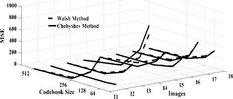
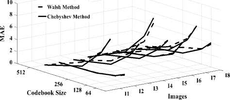
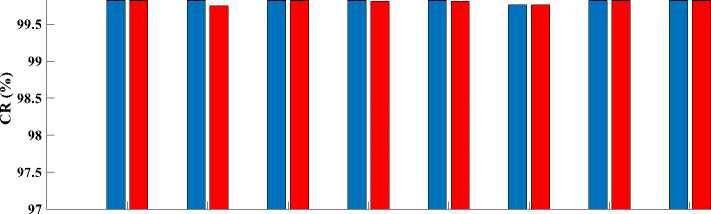
Fig. 5.a compares MSE according to the codebook size obtained in DWaT and DChT. It can be observed that error decreases gradually with increase in codebook size. DWaT gives a maximum error. When codebook size is 256, average MSE is 32.001 in DChT and 50.165 in DWaT. Fig. 5.b shows MAE versus codebook size obtained in DWaT and DChT. Here also DWaT gives maximum error. MAE nearest to zero indicates image quality is closest to the original image. Fig. 6.a compares PSNR obtained in DWaT and DChT with different codebook size. DChT gives maximum PSNR. Average PSNR is 35.78 dB in DChT and 33.107 dB in DWaT when codebook size is 256. As in the Fig. 5, when codebook size increases less error occurs and hence PSNR increases indicating better image quality. Fig. 6.b shows CR versus codebook size obtained in DWaT and DChT. Here, DChT and DWaT give almost the same values between 99.78% and 99.90%. Fig. 7.a and fig. 7.b show CT and DT obtained in DWaT and DChT respectively with different codebook size. Drastic difference is observed between DWaT and DChT. The fig. 8 compares against PNSR, MSE, MAE and CR obtained in DWaT and DChT with codebook size 256.

(a)

(b)

Fig.5. Three dimensions graphical representation of compression/ decompression using Walsh and Chebyshev methods. (a) MSE based on codebook size, (b) MAE based on codebook size.

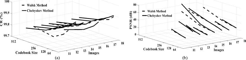
Fig.6. Three dimensions graphical representation of compression/ decompression using Walsh and Chebyshev methods. (a) CR based on codebook size, (b) PSNR based on codebook size

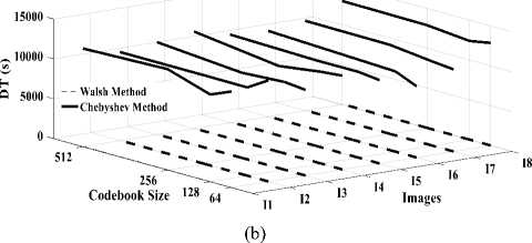
Fig.7. Three dimensions graphical representation of compression/ decompression using Walsh and Chebyshev methods. (a) CT based on codebook size, (b) DT based on codebook size.

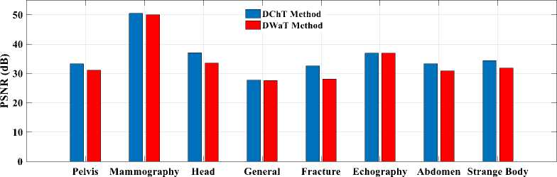
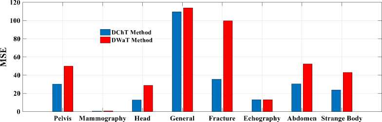
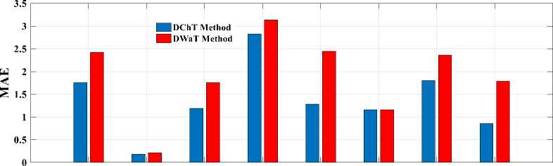
Finally, to see a real difference between compression by DWaT and by DChT, we have represented a bar chart. These charts are represented in Fig.8. In these charts, we have represented the difference between the eight tests images and two methods (DwaT and DChT) for a codebook size equal to 256. Thus, we find that on the chart representing the PSNR, the DChT and DWaT are slightly different and, on that of the CR, the two methods

(DwaT and DChT) are almost identical. On the charts of    two methods and conclude that the DChT gives good the MSE and the MAE we see a difference between our    parameters.

(a)

(b)

Pelvis Mammography Head General Fracture Echography Abdomen Strange Body

(c)

Pelvis Mammography Head General Fracture Echography Abdomen Strange Body

(d)

Fig.8. Parameters evaluation versus test images. (a): PSNR; (b): MSE; (c): MAE; (d): CR

In this work, we do not just simply use K-Means Clustering Algorithm to cluster the group of images and minimum Euclidean distance as in [24] or use LBG algorithm for vector quantization like in many works. We used the K-Means algorithm with the splitting method to optimize our codebook. Our Work is very adapted to the biomedical image because we can reconstruct an image without loss of information.

Now, we compared our compression method with two recent work. Ayoobkhan el al in [59] introduce a lossy compression method. The method in [59] denoted PE-VQ method uses the concept of vector quantization and prediction error. An optimal codebook is generated for VQ using a combination of two intelligent algorithms (artificial bee colony and genetic algorithms). Table 3 compares PSNR and CR obtained in introduce method (DWaT, DChT) and Ayoobkhan and al Method (PE-VQ) with codebook size 256 and 512. It can be observed that

PSNR increases gradually with an increase in codebook size. DWaT and DChT give maximum PSNR and equal to infinity when codebook size is 512. PSNR equal to infinity indicates image quality remains the same with the original image. The difference is observed between CR in our method and method in [59]. For example, average CR is 99:1 in our method and 80:1 in [59] with codebook size is 256. Our method outperforms and gives a good compromise between CR and PSNR. Fig. 9 shows the original image used for the comparison.

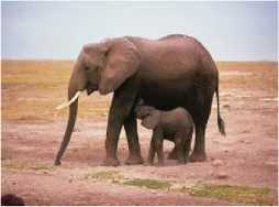
(a)

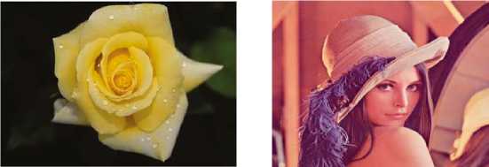
(b)                                             (c)

Fig.9 (a) Elephant; (b) Flower; (c) Lena [19, 59]

Table 3. Performance comparison (PSNR and CR) of the introduced method and [59] Method.

Method

Our Method

Ayoobkhan and al Method [58]

DWaT

DChT

PE-VQ

Codebook size

256

512

256

512

256

512

Parameters

PSNR (dB)

CR

PSNR (dB)

CR

PSNR (dB)

CR

PSNR (dB)

CR

PSNR (dB)

CR

PSNR (dB)

CR

Elephant

35.43

99:1

Inf

99:1

38.92

99:1

Inf

99:1

39.04

80:1

42.5

73:1

Flower

42.92

99:1

Inf

99:1

45.13

99:1

Inf

99:1

38.91

80:1

42.5

73:1

H. B. Kekre, and al in [19] used some parameters (MAE, Compression Ratio and AFCPV) to evaluate their algorithm. Table 4 gives the values of MAE and CR according to codebook size on the Lena color image. Table 4 compares CR and MAE obtained in our method and Kekre et al. method according to codebook size. Using KFCG and KMCG less error is obtained than an error in DWaT and DChT when the codebook size is 16.

MAE 8.36 and 8.34 is obtained for DChT and KFCG respectively when the codebook size is 32. MAE nearest to zero indicates image quality is closest to the original image. CR in DWaT and DChT is higher than in KFCG and KMCG. We obtained an average 99.90% and 99.34% in our method and Kekre and al method respectively for a codebook size 32. DChT outperforms DWaT and Kekre et al. method.

Table 4. Performance comparison (MAE and CR) of the introduced method and Method proposed in [19].

Codebook size	Parameters	Our Method		H. B. Kekre, and al Method [19]
		DWaT	DChT	KMCG+HWT	KFCG+HWT
16	MAE	10.12	10.07	10.09	9.32
	CR (%)	99.92	99.92	99.47	99.47
32	MAE	8.31	8.28	8.89	8.34
	CR (%)	99.91	99.90	99.34	99.34
64	MAE	5.51	5.44	-	-
	CR (%)	99.87	99.89	-	-

Thus in both comparison, our method has given the best result about related work. We can conclude that

IV. Conclusion

when the image is transformed with DChT or DWaT, and the codebook is calculated with a ML algorithm ( K -Means and splitting method), the compression is performed with very good parameters.

Our aim in this paper was to present a new scheme for biomedical color image compression. We present an optimal method for biomedical images compressing using orthogonal transform (DWaT and DChT) and vector quantization based on ML algorithm. ML algorithm (K-Means and splitting method) used to calculate and generate the codebook. VQ is applied on transform domain images. Using this scheme, image quality is obtained at an average CR 99.85%. MAE gives clear idea of image quality. At codebook size 256, an average MAE 1.38 and 1.89 is given for DChT and DWaT respectively. DChT outperforms DWaT in terms of PSNR, MSE and MAE. Computing time of DChT is very large compared to DWaT. As compared to Kekre method in [19] and Ayoobkhan method in [59] according to codebook size, DWaT gives less error and DChT gives least error among all with better image quality. The comparison demonstrates the effectiveness of the proposed scheme in biomedical color image compression. An extension to this work is to build a big data environment in order to simulate our proposed compression algorithm.