A Mathematical Model on Selfishness and Malicious Behavior in Trust based Cooperative Wireless Networks

Published Online September 2015 in MECS DOI: 10.5815/ijcnis.2015.10.02

The basic properties of wireless networks, and in particular the emerging networks like ad hoc and sensor networks, are often found to provide the leeway needed by the perpetrators, who carry out malicious attacks on such networks. Ad hoc networks are basically collections of several wireless mobile nodes which temporarily form a network which does not need to use any pre-existing network infrastructure and also there is no requirement for any centralized administration mechanism [1]. This enables wireless mobile users to communicate by forming an ad hoc network even in areas with no existing communication infrastructure or where the infrastructure is expensive or not convenient for use. Because of the lack of infrastructure, each node needs to operate both as a host as well as a router. This allows the forwarding of packets between such nodes which may not be inside direct wireless transmission range of each other. The nodes thus participate in an ad hoc routing protocol which allows any node to discover multi-hop paths to any other node through one or more intermediate nodes in the network. The positive essence of such networks is therefore the concept of co-operation and collaboration to collectively fulfill the broad requirements of a networking infrastructure. However, the constituent nodes comprising an ad hoc network also have to compromise with a number of limitations. They are basically characterized by severe constraint of resources including energy in the form of battery life, computing power, memory size and bandwidth. Also the dynamicity in such networks is another primary characteristic feature which complicates several aspects of communication. It arises because of different reasons including node mobility, topology changes, failure of nodes and also due to conditions arising out of the propagation channel. In particular the security aspect is made complex by features like openness to eavesdropping, unreliable communication, lack of specific ingress as well as exit points, and also topology changes because of node mobility and node failure [2].

An abstract consideration of the cooperative and collaborative behavior of ad hoc networks leads us to two important concepts, viz. trust and reputation. The notion of trust can be traced to its applications in social and societal studies, based on which it may broadly be defined as the degree of subjective belief that a given entity (may be a person, an organization or a node, in our case) behaves in accordance with a set of well-established rules and meets the expectations of other entities [3,4]. In civilized society the concept of trust assumes a fundamental position as far as human behavior is concerned and in majority of cases it is considered to be a major offence when a trusted entity performs a breach of trust. The concept of trust management finds an important place in computer security and is identified as a distinct component of network security services [5]. Analyzing, quantifying or proposing theory about trust and its management for societal behavior has been a tough proposition and it remains so even for computer networks. In ad hoc networks trust management becomes a crucial issue when, without any previous interactions, the nodes need to communicate ensuring a desired level of trust between them. It finds several applications in diverse decision making situations like authentication of certificates, access control, intrusion detection, key management as well as isolating misbehaving nodes to enable effective routing [6]. The concept of reputation is related to that of trust but has a slight difference in meaning and application. Trust emphasizes risk and associated incentives but reputation is concerned with a perception that gets associated with a node based on its past actions in the perspective of the existing or agreed upon norms [7]. Two other important notions that arise from an abstraction of the security scenario are malicious behavior and selfish behavior of the nodes [4]. An attacker in an ad hoc network primarily aims to disrupt the normal functioning of the network. In particular, most active attacks can be characterized as a method of subduing the basic tenet of collaboration that is so unique in such networks. The aim is to use as many nodes as possible to behave in a malicious manner. Selfishness may be characterized as the lack of cooperation by the concerned node. This may be seen as a direct implication of the resource limitations but it may be an indirect result of a malicious attack.

In this paper these fundamental ideas are explored and their role is analyzed in the perspective of ad hoc network epidemics. An epidemic model is proposed that considers the dynamics of an attack when the nodes try to cooperate and maintain an acceptable level of trust for communication. Section 2 establishes the basic assumptions and a mathematical formulation of the model. In section 3, equilibrium points of the system are obtained and also a basic threshold value called the basic reproduction number is found. A condition for the behavior of the system based on this condition is also established. In section 4, a stronger condition for the global stability of the equilibrium points is established. Section 5 analyzes several aspects of the behavior of the system using numerical simulations. The conditions obtained in the previous sections have also been validated using specific examples. Section 6 finally concludes the paper.

• II.    M athematical M odel

The consideration of a difference between the malicious and selfish behavior of non-trusted nodes leads us to use two different sub-classes in the epidemic framework. The attacker primarily aims to increase the number of malicious nodes. On the contrary, the requirement for an efficient functioning of the network is that the number of trusted nodes remains above a minimum threshold. The number of both malicious as well as selfish nodes needs to be controlled as their behavior determines the efficiency of the network, even though they behave differently as far as spreading the infection process is concerned. It needs to be emphasized that there may be infection in both malicious and selfish nodes. The participation of selfish nodes in spreading the infection may be less, and may even be negligible. This is because of the decrease in co-operative behavior from these nodes due to selfishness. The population in our model is partitioned into five compartments, viz. trusted, exposed-malicious, exposed-selfish, infectious-malicious and infectious-selfish. The difference between the exposed and infectious stages is only to model the fact that the nodes may spend some time in the process of becoming fully infectious. This will be context-dependent and may not be seen in many practical scenarios, where such a time gap may be negligible or even totally absent. Also between the process of being exposed and becoming infectious, a possible switch in behavior between malicious and selfish behaviors has been maintained as a consideration. This is only based on the fact that the identified behavior of the exposed nodes may have an error. In particular, the aim is to avoid proceeding with a scenario where a significant number of malicious nodes are identified as merely selfish. Also any node, irrespective of being trusted or non-trusted, may fail to function at any stage of the process. In the long run this fact can be modeled by a simple constant rate of removal for the nodes. The infectious-malicious nodes and the infectious-selfish nodes, however, have a higher rate of losing their functionality when compared to the other nodes. This assumption models the fact that infected nodes will ultimately stop functioning after some stage if not attended to, while selfish nodes will also tend to becoming isolated as they stop forwarding data. All new nodes added to the network are assumed to be initially trusted. This assumption models a behavior-based trust management framework, which is a reactive approach where the trustworthiness of a node is ensured by preloaded authentication mechanisms [8]. In such a case the behavior of each node is continuously monitored by the neighboring nodes to evaluate its trustworthiness. A node that behaves in an unauthorized manner, for example in its use of network resources, loses its trust as the neighbor nodes identify this behavior. Another assumption is that the nodes become exposed-malicious or exposed-selfish according to a certain probability which has a constant value in the long-run. The sum of the probabilities essentially has to be one. On the basis of these assumptions, the dynamics of the nodes between the trusted and non-trusted compartments is shown in Fig. 1.

The rate of addition of new trusted nodes into the network as well as that of the removal of non-functioning nodes from the network are both assumed to be a small positive constant, say ц. A bilinear incidence is assumed in both the cases of malicious as well as selfish populations which accounts for the fact that the spread of infection depends on the strengths of both the interacting populations.

For notational convenience, we take 1 for malicious (m) and 2 for selfish (s) nodes in the subsequent discussion. This makes system in (2) to appear as follows

dT dT = цTo- ц +

Z e j i j j = 1

)      2

T + Z y j i j

J      j = ¹

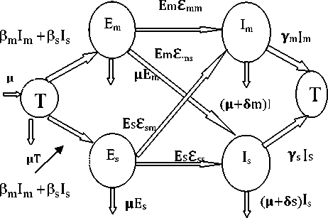
Fig. 1. Schematic diagram for flow of worms in mobile network.

r

2                 2

= p i Z e j i j T - ц+ Z^

A

Ei

к j = 1 J

d j = Z ^s ij^Ei ^{- (}ц ^+Y j ^{+ 5} j K-

where the total population size is where

N = T + Z E i + Z I j          (4)

i = 1        J = 1

The parameters p _m and p s represent the infectivity contact rates for the malicious and selfish infectious nodes, respectively. The long-term probabilities with which the trusted nodes become exposed-malicious and exposed-selfish are taken as p_m and p_s respectively where

p m + P s = ¹                    (1)

The rates at which the exposed-malicious and exposed-selfish nodes become infectious-malicious and infectious-selfish are represented by the respective parameters ^s mm ^{and S} ss .

The rates at which they change behavior and become infectious - selfish and infectious-malicious are respectively represented by s _ms and s sm . Further the additional rates at which the infectious-malicious and infectious-selfish nodes become non-functional are represented by parameters 5 _m and 5 s respectively. Finally the recovery rates are taken as у _m and у s for the infectious-malicious and infectious-selfish populations respectively.

The following systems of equations can be derived based on the transfer diagram in Fig. 1:

III. B asic R eproduction N umber A nd L ocal S tability F or I nfection -F ree E quilibrium

In this section the model is analyzed from a basic epidemic perspective. Firstly, the equilibrium points for the system are identified. Then an important threshold quantity called the basic reproduction number is defined and the variations in the behavior of the system based on this threshold are established. points after.

Theorem 3.1.

System (3) has a trivial infection free equilibrium at (T = T₀, E₁ = 0, E₂ = 0, I₁ = 0, I₂ = 0). Moreover it also has a unique endemic equilibrium (T*, E₁*, E₂*, I₁*, I₂*) where the infectious components are both positive while the remaining components may be non-negative. The endemic equilibrium exists when the quantities T 0 – 1 and G – H are of the same sign, where

p 1 ^£ 11 ^{( M +} £ 22 ) ⁺ p 2 ^£ 21 ^{( M +} ^ 12 ) ^{+ (} p l ⁺ p 2 ) ^£ 11 ^£ 21 M + P + Y i                 _

P 2          P l ^£ 12 ( M ⁺ ^ 21 ) ⁺ P 2 ^£ 22 ( M ^{+ £} ii ) + ( P i ⁺ P 2 ) ^2 ^ 22

P i ( M ⁺ S 21 + S 22 ) [                    M ^{+ P} 2 ⁺ Y 2                   .

g =       -----T p1 ( M + S21 + S22 )

and

— = M T - ( M + P m I m + P s I s ) T + ( / m I m + / s I s )

_H=        Y1        P1 ^s 11 ( ^p + ^s 22) ±P 2 ^s 21 (E± ^s 12) ±( P L±P2) ^s 11 ^s 2L

P 1 ^{(p + s} 21 ^+s 22 ) L                   ^{P + 5} 1 +Y 1                    _

₊ _______Y2________ ^p 1 ^s 12 ^{(p + s} 21 ^{)+ p} 2 ^s 22 ⁽ 4 ^{+ s} 11 ^{)+( p} 1 ^{+ p} 2 ^)s 12 ^s 22

^p 1 ⁽ Ц ^{+ s} 21 ^+s 22 ) _                   ^{ц + 5} 2 ^+y2                  .

dEm dt dEs dt dIm dt dIs dt

pm (PmTIm + PsTIs ) - (M + Smm + Sms )E ps (PsTIs + PmTIm ) - (M + Ssm + Sss ) Es (EmSmm + EsSsm ) - (M + Уm + Pm) Im

( ^Em ^S ms + ^Es ^S ss ) ^- ( M + Y s ^{+ P} s ) I s

Proof . To find the equilibrium points of the system, we need to solve the following set of equations:

^{ц T}0 ^{- (ц +} P 1 I 1 ⁺ P 2 I 2 ) ^{T +} Y 1 I 1 ^{+ Y} 2 I 2 = ^{0      (5)}

^p1 ⁽P 1^TI1 ⁺ P 2^TI2 ) ^{- (ц + s} 11 ^{+ s} 12 ^{) E}1 = ^{0      (6)}

Р 2 ( ₽ 2^Т12 + P 1^TI1 ) - ( ^ + ^£ 21 + ^£ 22 ) E 2 - 0      (7) where

• ^E1 ^£ 11 + ^E2 ^£ 21 ^- ( ^ + Y 1 + 5 1 ) I 1 ^- 0           ⁽⁸⁾

• ^E1 ^£ 12 + ^E2 ^£ 22 ^- ( ^p + Y 2 + ⁵ 2 ) I 2 ^- 0          ⁽⁹⁾

If we consider I₁ to be zero then from equation (8), both E₁ and E₂ need to be zero as the coefficients are both positive constants. Substitution of these values in (9) gives I 2 - 0 and consequently (5) gives T - T q . So, at this equilibrium both the infectious populations as well as the two exposed populations vanish, and hence it is called the infection-free equilibrium .

Next we consider the case when I₁ andI₂ are both nonzero. From (6) and (7) we have e * _- AE * where

A - P 2

p1

Ц + £ц +£ 12

Ц + £ 21 + £ 22

Substitution of this value in (8) and subsequent simplification yields 1 * _{- BE}* where

B - ^{£ 11 +} A ²¹                (11)

ц + § 1 +Y 1

Similarly (5) gives I 2 - CE * where

C - ^{£ 12 +} A ²²                (12)

ц+5 2 ^+Y 2

Putting these values in (6) and simplifying, we get

T*

¹ | Ц ^{+ £} 11 ^{+ £} 12 P 1 ( B ₽ ! + C ₽ 2

Further from (5) we get

_E * ₌         B^{( t}0 ^- 1 )

^{1   B(}P 1 ^-Y 1 ^{)+ c (}P 2 ^-Y 2 )

The other values have already been expressed as constant positive multiples of E ^* . So, these components together represent the endemic equilibrium

B p * + C p 2

_         P1         ^p1 ^£ 11 ^{(p + £} 22 ^{) + p}2 ^g 21 ⁽ B ^{+ £} 12 ^{)+( p}1 ^{+ p}2 ^)e 11 ^£ 21

^p1 ^{(p + £} 21 ^+£ 22 ) _                   ^{p +} § 1 ^+Y 1                  .

+       в2 p1£12 (p + £21) + p2£22 (p + £11) + (p1 + p2 )£12£22 p1(p + £21 +£22 ) _                 p + §2 +y2                 _ and

B ^Y 1 ⁺ c ^y 2

Y 1	p 1 £ 11 (p + £ 22 ) + p 2 £ 21 (p + £ 12 )+ ( p 1 + p 2 )£ 11 £ 21
p 1 (p + £ 21 +£ 22 )	Ц + § 1 +Y 1

,     Y2        .	p 1 £ 12 (p + £ 21 ) + p 2 £ 22 (p + £ 11 ) + ( p 1 + p 2 )б 12 £ 22
p1 (p + £ 21 +£ 22 )	Ц + § 2 + Y 2

If these quantities are denoted by G and H, then (16) holds when T q - 1 and G - H are either both positive or both negative.

A. Basic Reproduction Number

The basic reproduction number is defined as the number of secondary infectious nodes caused by an individual infected node during its infectious period in a population which is totally susceptible [9]. It is commonly denoted by R₀.The most important property of R₀ is that it acts as a threshold, such that if R q <  1then the infection dies out, and if R q <  1 , the infection persists. For epidemic models with multiple infectious classes, the basic reproduction number is defined by the spectral radius of the next-generation operator [10-13]. For epidemic models with heterogeneous population structure, the basic reproduction number can be efficiently determined by the local stability of the infection free equilibrium, that is, the dominant eigen value of the Jacobian matrix at the infection free equilibrium for models in finite dimensional space [14,15]. The infection free equilibrium for system of equation (3) is given as (T = T 0 , E 1 = 0, E 2 = 0, I 1 = 0, I 2 = 0). In this section, we drive the expression for R 0 by investigating the local stability condition of the infection – free equilibrium as follows:

The Jacobian for system (2) at the infection free equilibrium is given by

T, E_b E 2 - AE * , I 1 - BE * , I 2 - CE * )   (15)

Here T^* and E^* are given by (13) and (14). Now, this equilibrium point will exist only for non-negative values of E^* . The condition for this is as follows

_________ ^T0 ^-1 _________

( B P 1 + C p 2 ) - ( B Y 1 + C y 2 )

> 0

-Ц

J -   0

J 22

J,3

J 23

J 33 .

Where the following sub-matrices have been considered for the sake of notational convenience

J 13 ^-[- P 1^T0 ^+Y 1   ^- P 2^T0 ^+Y 2 ]

J 22 = diag

Г      2     )

>•+2^

I      j = l     J

Г     2      )

*-2‘2j l     j=l    J

As R_o =p ( FV ^{- 1} )

on solving, we get as in

^p1 P 1^T0    P 1 P 2 T 0

. ^p2 ₽ 1^T0  ^p2 P 2 T 0

^J32 =

^E 11

.E 21

^e 12

^E 22

^J33 = diag ^{[ -} ( ц + У 1 +3 1 )   ^- ( ц + У 2 ^{+ 3} 2 ) ]

If F represents the rate of appearance of

new

infectious nodes and V represents the difference of outward to inward flow of nodes into any compartment, then

^Fii =

^pi ⁽P 1 I 1 ⁺ P 2 I 2 ) T 0 ⁰ 0

and

^Vij =

^{(ц + E} i1 ^{+ e} i2 ) E i

- (ei1 + ei2 )Ei + (ц + Y j + 3 j )I j

_p + P1I1 + P2I2 -(Y1I1 + Y2I2)_

Differentiating partially w. r. to the infectious variables, we have

F =

0  P i P j T o

and

V =

Ц + Е ^Е У j = 1 — ^E j

ц+Y j +3 j

If we write the general form of above matrices, we

have

F =	"0	J 23"	and V =	" - J22	0  "
	. 0	0 _		.— J32	- J33 _

Taking the inverse we have

V-1

-J22

_ ^J33^J32^J22

-1

J 33

Ro = To z Pi z k=1   i=1

____________ Pi ^E ki _____________

Г       2     '

( ц + Y i ⁺³ i ) ^{p +} 2 ^E ij l      j = 1    J

On the basis of the above discussion and the definition of the basic reproduction number, the following result follows. It may be mentioned here that the result may be proved explicitly using linearization but we state the intuitive result directly in the following theorem.

Theorem 3.2.

The infection free equilibrium is locally asymptotically stable if R₀ <  1 and unstable if R o >  1.

Table 1 shows the corresponding behaviour of the system for different values of the basic reproduction number. The table values also point to the fact that the infection-free equilibrium is stable when the values of the basic reproduction number do not exceed the threshold value of one.

Table 1. Asymptotic Behaviour of System for Different R 0 Values

R 0	T	E m	E s	I m	I s	Equilibrium type
0.0760	1.0000	0.0000	0.0000	0.0000	0.0000	IFE
0.2281	1.0000	0.0000	0.0000	0.0000	0.0000	IFE
0.4561	1.0000	0.0000	0.0000	0.0000	0.0000	IFE
0.6842	1.0000	0.0000	0.0000	0.0000	0.0000	IFE
0.7602	1.0000	0.0000	0.0000	0.0000	0.0000	IFE
0.8363	1.0000	0.0000	0.0000	0.0000	0.0000	IFE
0.9883	1.0000	0.0000	0.0000	0.0000	0.0000	IFE
1.1404	0.7863	0.1756	0.1054	0.0302	0.0413	Endemic
1.2164	0.7371	0.2160	0.1296	0.0371	0.0508	Endemic
1.2924	0.6937	0.2517	0.1510	0.0433	0.0592	Endemic
1.3684	0.6552	0.2834	0.1700	0.0487	0.0666	Endemic
1.4444	0.6207	0.3118	0.1871	0.0536	0.0733	Endemic

In the next section a proof is provided for a more stronger condition about the stability of the infection free equilibrium when _Ro <  1 . copy.

IV. G lobal S tability C ondition F or I nfection F ree E quilibrium

In the previous section we had obtained an expression for the basic reproduction number and had used its definition to obtain an intuitive result about the behavior of the infection-free equilibrium. In this section the behavior of this equilibrium point is characterized in theorem 4.1. In subsequent discussion, the behavior of the other equilibrium point is also explored, which allows us to analyze the nature of the system when the value of the basic reproduction number exceeds the critical value.

Theorem 4.1.

The infection free equilibrium is globally asymptotically stable provided R o <  1.

Proof. Total population satisfies the equation

= ( ц Т „ -ц^- £ б j l j

J = 1

From (22) it is clear that — <  0 if R_o <  1 and dt           ⁰

• -l _{= 0} if and only if i . = o. Clearly, function L is dt                               ^j

positive definite over G and its time derivative is negative definite. So the infection free equilibrium is globally asymptotically stable. Further if R_o >  1 then ^dL >  o if dt

Ij >  o, i.e. the equilibrium is unstable if r₀ >  1.

In the next section different aspects of the behavior of the system are analyzed using numerical simulations.

where n _e ( o, t₀ ] . Here we take the domain as

G = {(T, E, I) :0 < N < To} where e = (ex E2 )t and I = (li I2 )T ■ Then the domain is positive time–invariant for the system (3).

We use the Lyapunov’s second method of stability in this section to show the global stability of the infection free equilibrium. Let L be a Lyapunov function which is a real valued function defined on G as follows

2          f      2     1

L ^Ji + Р + ^ Ij i = 1           I      J = 1     J

At infection free equilibrium (IFE), l ( ife ) = 0

and otherwise,

L ( x ^ IFE ) >  0 for all x e G

The time derivative of L is given by

• V. N umerical S olution A nd S imulation

In this section numerical simulations are used to highlight some aspects of the behavior of the system. These numerical experiments are aimed at both validating the analytical results that were obtained in the previous sections, as well as to bring forth the trust based aspects of the model which might have remained non-apparent during the epidemic analysis. The results are highlighted using the following four examples.

Example 1. In this example we highlight a scenario where the infection dies out in the system and all the nodes together provide a trusted environment to each other. Such a situation is conducive to an efficient functioning of the ad hoc network. The value of the basic reproduction number in this case is found to be R_o = 0.1404 < 1. It can be observed from Fig. 2 that the infection free equilibrium is asymptotically stable in this situation. This means all nodes become infection free in the long run thereby guaranteeing efficient communication.

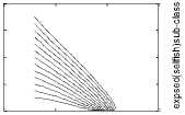
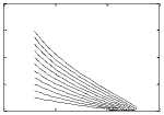
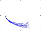
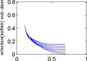
Example 2. In this example (Fig. 3) the stability results proved analytically in earlier sections is shown graphically.

dL       dE

= > £    - + dt          ij dt

I      i = 1    J

dI j dt

Putting the values of dEi      dI j from (3) in the dt      dt above equation and on solving we get,

dL dT = (P+YJ

22 t ZE k = 1 i = 1

___________Pi £ ki___________

Г 2    1

( ц + Y i ^{+ 3} i ) Ц + Е ^£ч I      J = 1    J

- 1

I J

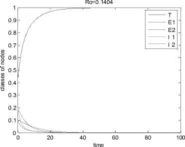
Fig. 2. Trusted environment in network when R o <1.

which on simplification using (18) gives

2     1

2 * 8 ( R o — 1 ) I j

J = 1     J

(Parameter values: P 1 = o.o5, p 2 = G.G5, £ц = G.G5, £ 1 = o.o4, £ j2 = o.o8, £ 12 = o.o9, Y 1 = o.5, Y 2 = o.5, P = o.o3, § 1 = o.o4, 3 2 = o.o4.)

3(a), Ro=0.1404

0.8

0.6

0.4

0.2

0.5

1.5

3(b),Ro=0.1404

0.8

0.4

0.6

1.5

0.5        1

trust

trust 3(c),Ro=0.1404

0.8

0.6

0.4

0.2

1 tust

0.2

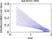
Fig. 3. Dynamic behaviour of non-trusted classes with respect to the trusted class when R o <1.

0.8

0.6

0.4

0.2

5(c),Ro=8.6039

0            0.5            1

trust

5(d),Ro=8.6039

trust

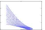
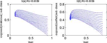
Fig. 5. Dynamic behaviour of non-trusted classes with with respect to trusted class when Ro>1.

(Parameter values: β = 0.05, β = 0.05, ε = 0.05, ε = 0.04, ε = 0.08, ε = 0.09, γ = 0.5, γ = 0.5, µ = 0.03, δ = 0.04, δ = 0.04.)

In this specific scenario all the four phase-planes that can be formed by the four non-trusted groups have been considered in the perspective of the trusted group of nodes. Here the value of Ro is 0.1404 which is less than 1, and hence all types of infection vanish and nodes form a trusted network, as shown in Fig. 3.

In Fig. 5 the phase planes of all the four non-trusted nodes have again been considered vis-a-vis the trusted nodes. The stability of the endemic equilibrium for the four non-trusted groups is shown in the perspective of the phase plane formed by them with the trusted group of nodes.

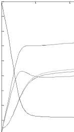
Example 3. In this example the opposite scenario is considered where the proportion of trusted nodes drastically decreases and makes it highly infeasible for the network to survive against any malicious attack. Here R₀ = 8.6039 > 1 which satisfies the condition for asymptotically stability of the endemic equilibrium. This fact is highlighted in Fig. 4.

Example 4. Again for the same situation considered in the previous example, the stability aspect is shown in Fig. 5.

0.9

Ro=8.6039

0.1

0.8

0.7

0.6

0.5

0.4

0.3

0.2

trust E1

E2

I 1

I 2

40        60

time

Fig. 4. Non-Trusted environment in network when R O > 1.

(Parameter values β = 0.9; β = 0.8; ε = 0.05; ε = 0.04; ε = 0.08; ε ₁₂= 0.09; γ ₁= 0.05; γ ₂= 0.05; µ = 0.05; δ ₁= 0.04; δ ₂= 0.04)

• VI. C onclusion

Appropriate estimation and approximation of epidemic spread in a network is important for preventing high-impact attacks. Lack of inclusion of important network properties in available epidemic models is still an issue that can be distinctly looked into for an improved model performance. Hence, inclusion of fundamental network and communication characteristics into the epidemic framework might be helpful. In this paper, a five-compartment differential epidemic model has been developed. It has been applied to analyze the impact of different abstract communication characteristics like trust, selfish behavior and collaborative communication on network epidemics in a wireless network. Long term behavior of the system was predicted in terms of two equilibrium points. A well-defined epidemic threshold for the system was obtained, and its significance in guiding the overall behavior of the system was established. Simulations were performed to test and verify the theoretical results under different sets of conditions. In future, the model can be extended to include the impact of different topologies of the network, or the impact of mobility of the wireless nodes.