A Method for Building a Mosaic with UAV Images

Published Online November 2010 in MECS

Compared with manned aircraft, using Unmanned Aerial Vehicles (UAVs) has many advantages [1]: 1) UAVs do not need a qualified pilot on board; 2) UAVs can enter environments that are dangerous to human life; 3) It is easy to implement high-risk and high-tech missions; 4) No need of permission for airspace control for low-altitude flights in most countries (such as P. R. China); 5) Lower costs of the platforms than that of traditional airplanes; 6) High resolution images and precise positioning data. As a result of these advantages, building Earth observation systems based on UAV platforms has become a hot topic throughout the world. Therefore UAV-based photogrammetry is becoming a popular field of research.

Although the UAVs can provide images with high resolution in a portable and easy way, the images only cover small parts of the interesting areas. For some surveying missions, we need a method to put all the sequence images together to make a larger image to check the quality of the raw data.

The distance from the camera to the target objects is very much greater than the motion of the camera between views, so the relationship between neighboring sequence images can be described by a homographic model [2], [3], [4]. However, when we use all the sequence images to create a mosaic which can provide us a larger view, the accuracy of the homographies may be affected by the accumulated errors (Figure 1).

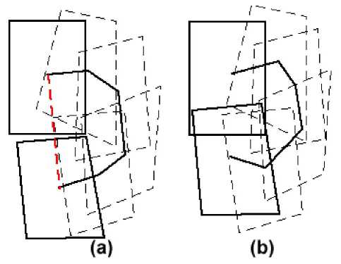
Figure 1. Accumulated errors cause poor alignment near the end of a loop. (a) the final image is not coincided with the first image, (b) a perfect mosaic with corrections.

In this paper, we introduce a two-step optimization method for mosaicking UAV sequence images. Firstly, overlap analysis of sequence images and some work of preprocessing should be done. Then stable features are extracted by using the SIFT (Scale Invariant Feature Transforms) algorithm, and these feature points should be matched. Thirdly, a local optimization method based on Extended Kalman Filter is applied to improve the homographies within local areas. Finally, a global optimization based on Levenberg-Marquardt algorithm is used to correct the position of each resampled image in the mosaic. The final results are shown in the section of tests.

• II.    H OMOGRAPHIC TRANSFORMATION COMPUTATION

• A.    Features extraction

A wide variety of scale and rotation invariant feature extraction algorithms have been proposed for detecting correspondences among images. Some experiments have been made to test the performance of existing feature extraction algorithms [5], and the results shows that the SIFT algorithm [6, 7] is better. So, in this paper, we use the SIFT algorithm to extract features from the sequence images (Figure. 2).

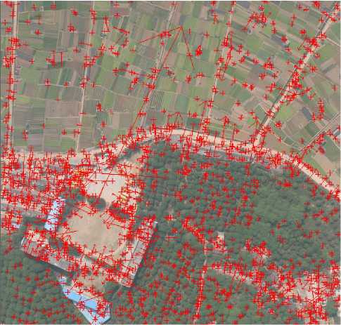
Figure 2. Feature points extracted by the SIFT

• B.    Perspective projection

A set of feature points can be extracted by the SIFT algorithm, and then we can match them. The next step is to compute the relationship between neighboring images.

The relationship between the two neighboring images can be considered as perspective projection, so the homographic transformation can be calculated by:

‘   m 1 x + m 2 y + m 3

m 7 x + m ₈ y + 1

‘ _ m 4 x + m 5 y + m 6 m 7 x + m ₈ y + 1

where ( x , y ) are the coordinates on image 1 and ( x’ , y’ ) are the coordinates on image 2, and M=[m 1 , m 2 , …, m 8 , 1]^T are the 8 parameters of the homographic transformation which can also be expressed as a 3*3 matrix denoted by:

M =

m ₁

m ₄

m ₇

m ₂

m ₅

m ₈

m ₃

m ₆ 1

So we can use at least 4 matched points to compute the transformation matrix.

• C.    Homography covariance estimation

Once the transformation matrix is computed, we require a measure of the estimation accuracy, and the here we can use the covariance matrix of the homography to measure the accuracy.

After getting a set of matched feature points, we can compute the covariance matrix by the way proposed by Hartley [8]. The matched feature points can be expressed as follows:

F = { { F F } { F 2 , F 2' } , - , { F n , F n '} } (3) Where F i = [ x i , y_t ] T , F_t = ^ x i , y i ^| . Firstly, we should calculate the Jacobian of the transformation from F to F ’ with respect to the 8 parameters of M , and then we can get a 2 n *9 matrix J . Secondly, the covariance of the residual ( C _Fi ) between each matched points should be computed, and because the residuals are uncorrelated, we can get the following matrix C _F :

CF = diag{CF1,Cf2,...,CFn} (4)

Finally, we can use matrix J and matrix C _F to compute the covariance matrix of the homographic transformation by the following equation:

Cm = (JT CfJF1 (5)

• D.    Attitude correction

The attitude of the UAV cannot be controlled as easily as that of the traditional large airplane, so the same objects on the neighboring images may not be displayed with the same shape, and the mosaicking result will be affected by this kind of distortion. Therefore, some correction should be applied before calculating the relationship between each pair of sequence images, and the attitude information can be provided by the Position and Orientation System (POS) on the UAV.

Figure 3 shows the relationship between a horizontal image and a tilted image [9], where S is the camera center, p is a horizontal image and po is a tilted image, c is the isogonic point, hchc is the isometric parallel, f is the focal length, point a is on the image p, the point ao is on the image po , rc and rco are the radius vectors, α is the angle of inclination, ϕ is a included angle between ca and hc, and ϕo is an another included angle between cao and hc. If the image po is rotated around hchc to the image p, point a and ao must be on the same line, and the correction can be described as:

δa = aao = rc -rco                         (6)

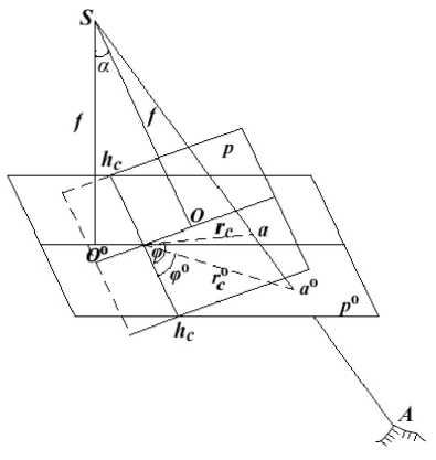
Figure 3. The relationship between a horizontal image and a tilted image

• III.    OPTIMIZATION METHODS FOR MOSAICKING

Suppose we have got the sequence images from two adjacent flight strips, and then we can compute the position of each image in the final mosaic through multiplying the current homography by all the previous homographies until the reference frame is reached. If the homographies are accurate, the mosaic will be perfect. However, there will be a drift between the last image and the reference image because of the accumulated errors. Therefore, we need to use some optimization method to improve the position of each image in the mosaic.

• A. Local optimization

We can divide the whole sequence images into several groups (Figure 4) by using overlapping degree analysis method [11], and each image in a group should have an overlapping area with the reference image. In this paper, the overlapping degree is about 60%~70%, we set six images in a local group (shown as group A and B in Figure 4). Then a local optimization based on the Extended Kalman Filter [12] is used to improve the homographies within a local area. The homographies corrected in this step can be used as initial values for the

The relationship between r_c and r_c ^o is:

^rc ^o

f grc

f - rc sinϕsin α

Therefore,

δ a

r _c

,0

r _c

rc sinϕsinα f - rc sinϕ sin α

r _c ^{o 2} sin ϕ sin α f + r _c ^o sin ϕ sin α

The tilted image can be corrected by (8).

E. The reference plane

The first image of the first flight strip can be selected as the reference plane during the process of mosaicking. However, the distortion may be accumulated larger and larger with the increasing number of sequence images. Therefore, a proper reference plane should be selected to decrease the accumulated distortion, and the distortion can be distributed equally to each sequence images.

The final result is a just mosaicking image, so the reference plane can be selected randomly. Here we can choose a dynamic plane as a reference. For example, when we are processing the first and the second image, an average plane can be chosen as the reference, and the this plane can be calculated by using the average values of each pair of corresponding points. When we put the third image into the mosaic, we can calculate an another average plane with the result made by the previous two images and the third image, and this is a new reference plane, and the rest can be done in the same manner [10].

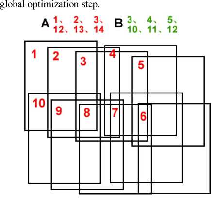
Figure 4. Groups of secquence images. With the analysis of overlapping degree, here we devide these two flight-strip sequence images into 3 groups denoted by A, B and C. The overlapping degree in our tests is about 60%~70%.

We suppose that the first image, denoted by I 1 , in a group is the reference image, and the last image in a group is I n . The relationship between an image and the reference image can be expressed as:

k

Mk1 = ∏M(i-1)i                   (6)

i = 2

where M _{k 1} means the relationship between image I k and the reference image I 1 . The a priori state vector will be composed by the n -1 transformations which align the n -1 images with I 1 and can be defined by:

x ^- = [ x 1 , x 2 ,..., x n - 1 ]^T = [ M 12 , x 1 g M 23 ,..., x n - 2 g M ( n - 1) n ]^T(7)

where the operator “ g ” is the product of two 3*3 homographic matrices, and the result is expressed as a vector.

The prediction equation and the covariance matrix can be expressed as:

xi = xi-1 gM i (i+1)

Cx = AC AT + WC_  WT xi            xi-1                  M i (i+1)

where matrix A can be obtained by computing the Jacobian of (8) with respect to the state vector and matrix W can be got by computing the Jacobian with respect to the variables of M i ( i _{+ 1} ) .

The measurement equation is defined by:

M_H = Hx = I X i - 1                       (9)

9 x 9 9 x 1

To update the state vector we can use the following expression:

x = x ^-+ K ( M 1( i + 1) - Hx ^- )                (10)

where K is the gain matrix. Finally, the relations among the images involved in the group can be updated with the measurement.

B. Global optimization

After optimizing the parameters within local areas, we need to use bundle adjustment to improve all the homographies globally. This step can solve the problems caused by the accumulated errors. All the sequence images are added to the bundle adjuster one by one, and the parameters can be updated by using the L-M (Levenberg-Marquardt) algorithm [13].

The objective function we use is a sum squared projection error. Each feature point is projected into every image in which it matches, and the sum of squared distances is minimised with respect to the parameters of the homographies. The squared residual can be computed by:

dk = d 2(F, Fp) + d 2( F, Fk)

where F_p^k_ji is the projection from image j to image i of the feature point corresponding to F_i^k , and we can use the following equation to compute F_p^k_ji :

F  = M jF(12)

The error function is the sum over all the images of the squared residuals:

n

D(M) = ZZ Z dk(13)

i = 1 j e I ( i ) k e $ ( i , j )

where n is the number of images, I ( i ) is the set of images matching to image I , S ( i , j ) is the set of matched features between images i and j .

This is a non-linear least squares problem which can be solved by using L-M algorithm. The iteration expression can be defined by:

Ф = (JT J + AI)-1 JT d(14)

where Φ are the corrections of all the parameters, d the squared residuals, J ^T J and J ^T d can be computed by:

(JT j )i,j= z ke $ (i, j)

n

Φ i

d d k T d d k

(JTd)i=ZZ z i=1 j eI (i) k e $ (i, j)

Φ

j(15)

ddk T, ij dk

Φi

This iterative process needs initial values which can be provided by the local optimization step. The detailed step of the L-M algorithm can be described as:

• (1)    set k =0, and compute the initial transformation matrix M _i ^k ;

• (2)    calculate the error function D( M _i ^k ) , and the get D( M ) ;

• (3)    use formula (15) to compute J ^T J and J ^T d , and then compute Φ using formula (14);

• (4)    if D( M ^k ) <  T ( T is a threshold), go to step (6), otherwise compute M ^{k + 1} and the error function D( M ^{k + 1});

• (5)    if D( M ^{k + 1}) <  D( M ^k ), we set k = k +1 and decrease the value of A , and then turn to step (2), otherwise the transformation matrices should not be updated, and set M ^{k + 1} = M ^k , and increase the value of A , then go to step (4);

• (6)    over.

• IV.    T EST RESULTS

  We use 10 sequence images from two fight strips in the test, and each fight strip includes 5 images. The resolution of each original image is 2592*3888. We take images No. 4 and No. 5 for example to show the processing results. Figure 5 shows the raw image No. 2, and Figure 6 shows the result of attitude correction with the POS information collected by the UAV.

The first step is the attitude correction for all the sequence images with the information provided by the POS, and then all the images can be similarly considered as horizontal images. The second step is the features extraction, we use the SIFT algorithm to extract features from each image in the sequence set, and then the feature points will be matched. Perhaps there are some wrong matches, so the wrong matches should be removed before calculating the homographies. Then, the local and global optimization methods described in this paper should be done to optimize the homographies between neighboring images, and finally we can put all the resampled images computed with the optimized homographies together to build            a            large            mosaic.

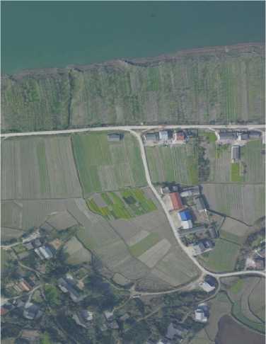
Figure 5. Image No. 2

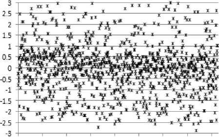
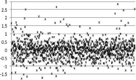
Figure 7 shows the residuals of x and y of each corresponding points on the two images before optimization process. Figure 8 shows the residuals of x and y of each corresponding points on the two images

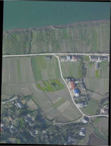
Figure 6. Attitude correction of Image No. 2

after local optimization, and Figure 9 shows the final residuals. Figure 10 shows the final mosaic by using the steps described in this paper.

Дх RMS=1.1638

Ду RMS=0.5683

О 1-Ю   280   420   560   700   840   980   1120

Figure 7. The residuals of x and y of each pair of corresponding points on two neighbouring images before optimization process.

О 140   280   420   560    700    840   980   1120

-г

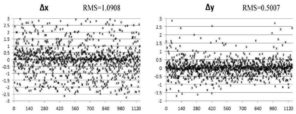
Figure 8. The residuals of x and y of each pair of corresponding points on two neighbouring images after local optimization process.

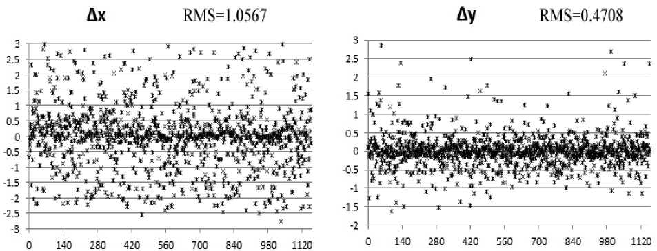
Figure 9. Final optimization results.

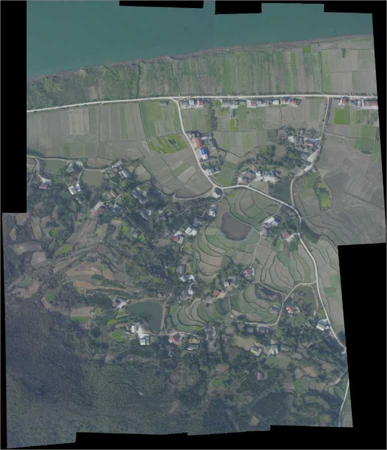
Figure 10. The final mosaic

• V.  C ONCLUSIONS

  Figure 6 shows the result of attitude correction, and the distortion caused by the attitude of camera is corrected after this step. Compared with Figure 7, we can see that in Figure 8 the residuals of x and y between corresponding feature points are improved by the local optimization process, and the RMS of x and y are reduced from 1.1638 and 0.5683 to 1.0908 and 0.5007. In Figure 8, we can see that the residuals are further improved by the global optimization step, the RMS of x and y are reduced to 1.0567 and 0.4708. The final mosaic shown in Figure 10 denotes that this two-step optimization method is suitable for sequence images mosaicking.