A methodology for automated labelling a geospatial image dataset of applicable locations for installing a wireless nodal seismic system

Seismic survey is a developing discipline of geophysics, which has a number of both scientific and practical applications. Seismic survey is involved in the search and exploration of mineral deposits [1–4], monitoring of urban and industrial facilities [5–7], in the construction of dams, bridges, buildings, etc. [8, 9], in the construction of roads, pipelines, subway tunnels, etc. [10, 11]. In addition, seismic survey can be used itself to find applicable locations for seismic monitoring stations [12].

Currently, the use of wireless nodal seismic systems has become widespread in seismic survey discipline. The obvious advantages of wireless nodal seismic systems compared to wired seismic systems (autonomous operation, uncomplicated installation and dismantling) justify their application potential in seismic survey. The design features of wireless seismic sensors [13–22] makes the installation procedure with much less time and labor consumption compared to the installation of a wired system:

it is enough to provide contact of the module’s sensors with the ground to make seismic measurements available. However, difficulties in installation of wireless seismic modules can be related to difficult transport accessibility of the target area where seismic survey procedure is planned.

In this work we consider a seismic nodal network consists wireless seismic sensors MTSS-1001 [23] with the bandwidth in range of 1 to 300 Hz that could be installed on hard and soft surfaces. The size of the sensor is 48×173 mm, the mass is 0.38 kg. The sensors in nodal network should be mounted at a distance of 100 m or more from each other. The sensors is able to wireless data transfer using WiFi with 120 kBits/s speed [24].

The procedure for delivery and installation of nodal network modules actualizes another key problem of search for applicable locations for seismic modules installation. At the same time, the design features of wireless seismic modules determine the specific properties of surfaces applicable for modules installing, which, in turn, determines the types of surfaces applicable for modules installing. The search for locations available for installation of modules can be performed by analyzing the available information about the surface in a specific geographic location where the wireless nodal network is planned to be installed. The information about the surface includes vector data of objects’ georeferences on the surface obtained from geographic databases, digital elevation model (DEM) data, as well as analysis of georeferenced raster images or geospatial images (satellite or aerial) of surface in the location of interest. Last kind of the data is of greatest interest from the analysis point of view. While vector data by itself may be missing or may be out of date, available DEM data may have inappropriate spatial resolution, geospatial images (especially satellite images) have the whole Earth coverage, relatively high spatial resolution and up to date. Geospatial image analysis methods require representative datasets, which contain features that are relevant to a particular class of underlying surface. Moreover, international [25] as well as Russian standards [26] states the principles of data quality for machine learning algorithms. One of the most important principle is data relevance that means that all the classes in the dataset really represent the real objects of interest, as well as all the samples in the dataset really correspond to the classes. Another requirements of data representativeness means that dataset contains all the classes of interest as well as the classes are represented by a wide range of specific parameters (in the case of geospatial images, dataset should contain images of various geographic locations, dates of obtaining images, wide spectral range). Obtaining satellite images in various spectral ranges is currently widely available at various dates via publicly available resources on the Internet. In this work, we consider the method for creation multispectral satellite images dataset.

The wide range of tasks and applications of seismic survey also determines the wide geography of locations where it is possible to install a wireless nodal seismic system, and, accordingly, a wide range of classes of underlying surfaces. This substantiates the urgency of development of a universal system of classes of the surfaces that are applicable for seismic modules installation for various geographical locations.

It should also be noted that the classes of surfaces that are applicable or non-applicable for installing seismic modules inherently represent classes of surfaces on the ground, which include wooded areas, various types of soil, agricultural land, urban development, etc. Therefore, collecting data from these surfaces might be of independent research interest (e.g., for feature to specific classes correspondence research). Such data themselves can be used in a wide range of other tasks of geospatial image analysis.

Seismic survey is usually carried out over large areas (of the order of several tens of squared km). Such territories usually contain a large variety of objects that need to be georeferenced with high accuracy. This is a labor- intensive procedure that requires automation. At the same time, there are many large geographic or spatial databases (DB), which contain a big number of objects that have high accurate georeferences. The examples of spatial DBs are community supporting OpenStreetMap (OSM) [27], WikiMapia [28], commercial Goggle Maps [29], Yandex Maps [30], etc. Georeferences of the most of the objects in such DBs, in turn, are carried out with high accuracy.

Another advantage of spatial DBs is the presence of georeferencing of the most important objects (residential settlements, industrial and transport infrastructure) even for sparsely populated and hard-to-reach locations. Therefore, the use of information from spatial DBs is promising for automating the labelling process. On the other hand, the systems of surfaces classes containing in spatial DBs have usually been developed based on the purposes of logistics, commercial and civil use. Therefore, GIS classifications require to be mapped to a system of classes of surfaces that are suitable for installing seismic modules. Another problem that may arise during this mapping is multiple labelling of the same object that also should be processed properly.

The paper discusses the development of a methodology for automated labeling of satellite images. The distinctive features of the developing methodology are use of spatial DB vector data for an accurate georeferencing objects on the satellite images, as well as the developing of mappings from spatial DB classes to a specific system of classes of the surfaces that are applicable for seismic modules installation, that automates labelling of the georeferenced area. In this work, we use OSM vector data as labels of spatial segments due to its free availability comparing to commercial spatial DBs and its data completeness and geographical coverage comparing to another community supporting spatial DBs (e.g., WikiMapia). It is also worth noting that in this work we are focused only on class names consistence.

1.    Related work

The use of UAVs in the task of controlling wireless nodal seismic systems is a relatively new discipline. Sudarshan et al [31] considers a seismic network, where each node is mounted on a separate UAV that perform mounting the sensors, gathering seismic data and deliver seismic module back. The wireless data transfer is not considered. The work [32] considers the aspects of using UAVs to gather seismic data of buildings foundations made of concrete. The work [33] considers the aspects of delivering and mounting wireless seismic nodal system using UAVs comparing to wired odal system. The work [34] describes an architecture of wireless geophone network. The authors test various parameters of IEEE 802.11ac and IEEE 802.11ad wireless data transfer protocols. All these works do not consider the task of identification the suitable for seismic module installation areas.

The work [35] considers an approach to aerial survey on the terrain applicable places to mount wireless nodal seismic system by heterogeneous group of UAVs. The work [36] considers the task of data collection from the modules of the wireless seismic nodal system. The works on the identification of suitable locations using geospatial data for installing sensors are also not widely represented in the literature. The work [37] is devoted to identification of agricultural land to mount soil sensors using satellite images. The result of this work, that is the most applicable to the tasks of the current work is revealed variability of the multispectral image features in the same surface class (soil) in different locations and image survey dates. This substantiates the need of developing methodologies for satellite images datasets collection.

Other works devoted to aerial and satellite images datasets consider various tasks of image analysis and types of considering surfaces. It is worth to highlight the peculiarities of the dataset collection methodologies in the related work. The authors of [38] consider flood areas identification using WorldView-2 satellite RGB and NIR images of areas in India and Singapore. The images have 2 m/pix. spatial resolution and 512×512 size. The authors performed manual labelling of 100 images using the developed by the authors software. Gonçalves and Lynch [39] considers RGB satellite images form WorldView-3 (size is 784×784, spatial resolution 1.24 m/pix.) of the Antarctic ice cover of sea. The authors performed manual labelling of the satellite images. The work [40] is devoted to Sentinel-2 satellite multispectral images (10 spectral bands, spatial resolution is 10 m/pix., images size is 10980×10980) of the crop collection in an interval from 2017-09-01 to 2018-09-01. The authors used the data provided by the farmers as labels with additional expert verification. Pan et al. [41] used Landsat 7/8 и Sentinel-2A/B imagery of Henan Province in China in a period from 2018-9-1 to 2019-9-1 in order to map winter crops. Pyo et al. [42] considers dataset of 17600 128×128 RGB aerial images with spatial resolution of forests with spatial resolution 0.25 m/pix. The images were obtained from 2018 to 2019. The images were labelled manually. The authors of [43] collected Sentinel-2 Water Edges Dataset (SWED) in order to perform coastline identification. The data was obtained in a period from 2017 to 2021. The dataset contains 98 256×256 images. The distinctive feature of this work is the development of an original classification of the coastline types that was used during labelling of the images. The main objective of the work [44] is satellite images super-resolution. The authors collected pairs of images of the same places with low (Sentinel-2, 10 m/pix) and high (PlanetScope, 2.5 m/pix) resolution, obtained at 2021 and 2022 from various geographic locations. The work does not consider labelling procedure due to super-resolution task does not imply that. Tripp et al. [45] collected a Sentinel-2 multispectral image (size is 10 980×10 980resolution is 10 m/pix.) as a part of flood on beaches monitoring task. The labelling of the data (two classes of interest – “Water” and “Not Water”) is performed using Semi-Automatic Classification

Plugin in QGIS software. The work [46] considers semantic segmentation of surfaces on satellite images with spatial resolution of 1 m/pix. The authors manually labelled one 10140×10120 image of Bronnitskiy forestry, which was divided into 64 square parts.

As a result, the works, where georeferenced images labelling is addressed, mostly consider manual labelling. The automation of labelling process using has a minor spread.

Due to modern spatial DBs contain detailed and accurate georeferenced vector data for a large number of objects, it is promising to use this data, such as OSM, to ease and accelerate labelling of geospatial images. Apart from strictly usage of georeference data from spatial DBs in labelling geospatial images, some works are of interest the GIS data processing, due to the problems of GIS classes and specific task classes inconsistency, GIS data absence and the mistakes in GIS labeling. One of the main objectives of such methods is to determine, how georeferenced objects (nodes, lines, polygons) [47] are related to a specific class of the surface, how to map one class of GIS data to another or how to determine area of some classes (e.g., industrial territory) using objects of other classes (e.g., buildings).

OSM has the original hierarchy of surface classes that is determined by logistic, land use commercial, civil and others contiguous purposes. That rises a specific task of adapting OSM classes to the classes corresponding to specific tasks. The work [48] considers various GIS data harmonization and adaptation in landcover mapping task. Fonte and Martinho [49] propose an original approach to comparison of GIS Urban Atlas OSM. This approach implies adaptation and harmonization of Urban Atlas and OSM hierarchies of classes. Patriarca et al. [50] consider the problem of OSM data consistency. The authors propose a method for OSM labeling verification, based on sequential and hierarchical processing of OSM data. Li et al. [51] considers using OSM as an additional source of labels of wastewater reservoirs (total object number is 4187) in order to label Sentinel-2 multispectral images. The dataset is part of deep learning pipeline of wastewater reservoir detection. In [52] the authors consider some technique that determines residential territory using OSM objects and Sentinel vegetation map. Ludwig et al. [53] consider the similar task of identification of green spaces using OSM objects and Sentinel-2 imagery. The authors of [54] propose an approach for OSM labelling assessment using deep learning. The work [55] is devoted to the problem enhancement of deep learning geospatial images segmentation using OSM. Li and Zipf [56] consider OSM data to label buildings on high-resolution satellite images in Mozambique and Tanzania. The authors formulate three types of errors inherent to OSM based on analysis of the obtained vector labels: incompleteness, alignment errors, and rotations. These errors arise due to the relatively high resolution of the considering satellite images. The work [57] considers gathering and labelling of Sentinel-2 satellite images dataset. The authors took labels from OSM (12 classes in total) without any supplementary processing of them. The authors do not process multiple labelling of the same objects. As a result, the dataset consists of 137045 images, of surfaces of 3.7 km2 and OSM labels for each image.

The survey of the related work has revealed the following uncovered problems of geospatial datasets labelling:

• 1.    Geospatial image analysis in a specific task of applicable surface identification for seismic modules installation has minor coverage in a scientific literature;

• 2.    The woks on datasets creation do not entirely fulfil the advantages of spatial DB labeling: usually only a few of OSM classes are used in labelling, the works on mapping OSM classes to the specific subject area, that require to restructure OSM class hierarchy, is not presented in a literature devoted to the dataset labelling. The works devoted to using OSM data as labels do not process;

• 3.    The works devoted to OSM class hierarchy restructuration mostly consider the mapping between OSM classes and classes of other spatial DBs. The aspects of OSM class hierarchy restructuration to the purposes of raster images labelling are not considered.

2.    Materials and methods 2.1.    Description of the steps of the methodology

The methodology of satellite images automated labelling described in the current work uses aper discusses the development of a methodology for automated labeling of satellite images. The distinctive features of the developing methodology are use of spatial DB vector data for an accurate georeferenced objects on the satellite images, as well as the developing of mappings from spatial DB classes to a specific classification of the surfaces that are applicable for seismic modules installation, that automates labelling of the georeferenced area.

The proposed methodology for collecting and automated labelling of satellite images consists of the following steps:

• 1.    Analysis of the subject area and development of a system of surface classes applicable for installing seismic modules;

• 2.    Analysis of the OSM map features classification. Development of a procedure for mapping objects and OSM classes into the applicable surfaces classes;

• 3.    Determining of requirements for geospatial images that meet the conditions of relevance to the task of identifying applicable areas for installing seismic modules;

• 4.    Obtaining OSM geospatial data;

• 5.    Obtaining satellite images;

• 6.    Mapping OSM objects into applicable surfaces classes;

• 7.    Performing an analysis of the results.

• 2.2.    Description of the surfaces classes considering for seismic modules installation

Further sections are devoted to revealing of the key aspects of the presenting methodology.

In order to fulfil the condition of data relevance to the specific task of identifying a suitable surface for installing seismic modules, it is necessary to determine the system of classes of corresponding surfaces properties related to this task. The considering system of classes is derived from the analysis of the expert survey and the analysis of design features of wireless seismic modules [58], as well as analysis of information about the specific geographic location where the wireless nodal seismic system is planned to be installed. The system of classes is presented on Fig. 1.

In this work, we consider common types of surfaces that are derived from a survey of experts and analysis of the design features of common seismic modules [13–22].

The content of each class of the considering classes shown on Fig. 1 are following:

• 1.    The “Water” class contains all the water surfaces: ponds, rivers, seas, etc.;

• 2.    The “Transport” class contains roads with various surfaces, as well as railways;

• 3.    The “Buildings” class contains areas of urban, industrial, commercial development;

• 4.    The “Water” class contains areas of natural and artificial reservoirs;

• 5.    The “Low Bushes” class contains areas covered with low vegetation, shrubs and grasses;

• 6.    The “Forest” class contains areas covered with trees;

• 7.    The “Ground” class contains areas covered with sand, bare soil and rocky surfaces;

• 8.    The class “Wetlands” contains areas of the surface of swamps – bogs and peat bogs.

The next significant aspect of the developing system of classes reflects the possibility of installing a seismic module on the surface. This aspect is expressed by a binary feature {suitable, unsuitable}, which label each surface class in the classification as suitable or unsuitable for installing a seismic module.

Some of the considering surfaces are unsuitable for seismic modules installation regardless to any other property. The developing system of classes contains one such class – “Water”. The other unsuitable surfaces are defined by a distinctive property – presence of economic, municipal, logistic and other human activities on a certain area. This feature serves to distinguish the surfaces whose properties allow the installation of seismic sensors. At the same time, the human activity on this surface makes it impossible to use this surface for installation seismic sensors. The examples of such properties are “Transport” and “Buildings”. In addition, it is of some interest to isolate such surfaces in order to study the differences in properties that can be extracted from images for those surfaces on which economic activity is carried out and those on which it is not carried out.

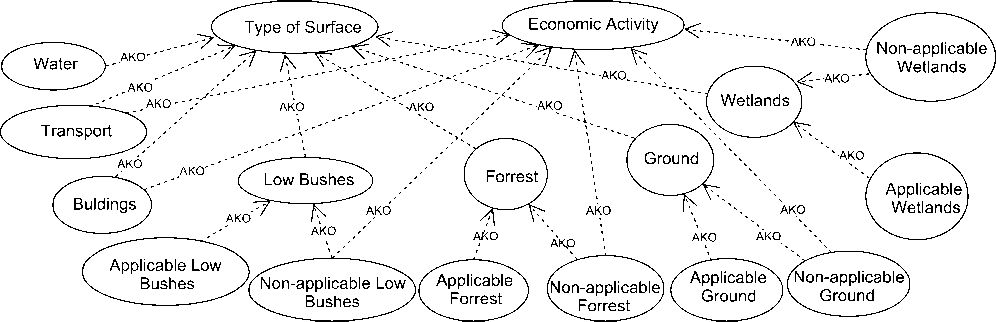
Fig. 1. Classes of the considering surfaces. Arrows AKO (A Kind Of) express the relationship between a class and a more general class

Applicable surfaces, on the other hand, in the developed system of classes are characterized by the properties of surfaces that explicitly determine the possibility of installing seismic modules on it and the absence of economic activity on them. Fig. 1 shows that some classes of surfaces: “Ground”, “Low Bushes”, “Forest”, “Wetlands” intersect for suitable and unsuitable surfaces, which is determined by the attribute “Economic activity”. The identification of additional subclasses of suitable and unsuitable surfaces for these classes is advisable, from the future image feature research point of view.

Now we consider the features that can characterize the described classes of surfaces that are suitable and unsuitable for installing seismic modules. The above mutually exclusive lists contain the same class names (soil, rocky surfaces, agricultural land, which can also be classified as soil). Therefore, additional characteristics are needed to differentiate them:

• 1.    The properties of surfaces that explicitly determine the possibility of installing seismic modules on it that is determined by GIS data (areas of residential buildings, industrial facilities, etc.);

• 2.    Data obtained directly from multispectral images of the area. These data include the brightness of pixels belonging to the corresponding multispectral bands. The values from different ranges of the multispectrum can, both in themselves, characterize one or another class of surface, as well as can be used to calculate specialized spectral indices (NDVI, NDBI, etc.) that characterize specific surfaces. This paper examines the multispectral range of satellite images from the Sentinel-2 database.

• 2.3.    OSM class hierarchy analysis

The resulting classes of the developed system of classes of the surfaces considering for seismic modules installation are the following: “Transport Infrastructure”, “Buildings”, “Water”, “Applicable Low Bushes”, “Non-applicable Low Bushes”, “Applicable Forest”, “Non-applicable Forest”, “Applicable Ground”, “Non-applicable Ground”, “Applicable Wetlands”, “Non-applicable Wetlands”.

OSM Map Features [59] (Fig. 2) is a class hierarchy of georeferenced objects. This is a tree-like hierarchy with the direct relations of the form (class, subclass). It is worth noting that the depth of the hierarchy is not limited.

The OSM class hierarchy had been developed for the commercial, municipal, and logistics tasks, not for the specific task of identification of applicable surfaces for installing seismic modules. Therefore, OSM class hierarchy cannot be directly mapped into another class hierarchy. Mapping procedure requires thoroughly comparison of the OSM and the target class hierarchy properties. In addition, the peculiarities of the OSM class hierarchy make it completely not feasible to separately map classes within one level of the OSM hierarchy to some class in the target hierarchy. For example, it is impossible to perform directly mapping all subclasses of the class “Natural” [60] into the class of surfaces applicable for installing modules (due to class “Natural” contains water surfaces). Therefore, it would be more appropriate to consider pairs (class, subclass), e.g., a pair (natural, scrub) as a unit of mapping to a class of applicable surface from the hierarchy. In addition, inspection of real combinations showed that not all pairs (class, subclass) could be directly mapped to the class system of applicable surfaces. Therefore, if not all the objects labelled by the pair (class, subclass) can be mapped to a single class of surfaces applicable for installation, it is necessary to map each distinct object labelled by this pair to the corresponding class of applicable surfaces.

It is also worth noting that the classes in the OSM hierarchy are not mutually exclusive. This means that the same object can be labelled by different classes. For example, different classes are combined in the same georeferenced objects (“amenity” and “building”, or “shop” and “building”). Moreover, there are no limits to the number of classes that can label to the same object.

Labelling objects in OSM is done by the community, that leads to the following common problems: la- bels do always not correspond to the recommended OSM class hierarchy structure; OSM database contain a large number of user defined classes that duplicate the OSM classes, which also complicates mapping procedure between two class hierarchies. It is also worth noting that community labelling and weak control over the labelling process and results leads to large number of mistakes. These mistakes also need to be processed during mapping from the OSM class hierarchy to the classes of applicable surfaces.

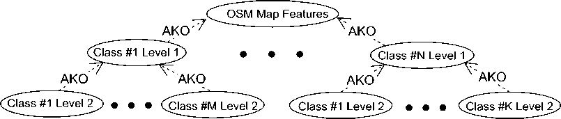
Fig. 2. Structure of OSM classes Arrows AKO (A Kind Of) express the relationship of a class to a more general class

The revealed problems of OSM class hierarchy define the main principles of OSM classes processing during mapping procedure:

• 1.    Consideration of combinations of OSM classes obtained in specific geographic locations, where satellite images are received. This is driven by the need to limit the total number of OSM classes;

• 2.    Detailed inspection of individual objects is required to identify valid correspondences between OSM classes and suitable surface classes, as well as to handle possible OSM labeling errors;

• 3.    Obtaining all possible values of OSM classes that label a single object in order to process multiple OSM labelling and avoid collisions when reducing it to a system of classes of suitable surfaces.

• 4.    Performing analysis of classes intersections.

• 2.4.    The procedure for constructing mappings of OSM classes into applicable classes

for seismic modules installation

In order to use OSM georeferences of objects as spatial segmentation in the task of labeling dataset of applicable surfaces for seismic modules installation, it is needed to map OSM classes and objects into the developed classification (Section 2.2). The mapping procedure consists of the following steps:

• 1.    Obtaining georeference data from OSM using Overpass API [61]:

• •    Filtering nodes objects [62] due to such objects do not contain useful information about spatial objects on the terrain;

• •    Converting OSM open way objects [63] such as waterways and roads OSM area objects [64] by adding width parameter to an open way object. The width value is based on the accepted minimum value of 10 m that is enough to cover area of roads and rivers on 10 m spatial resolution satellite geospatial images.

• 2.    Analysis of combinations of OSM classes (class, subclass) for compliance with the classes of suitable surfaces. This procedure is performed in two steps:

Construction of all combinations of top and second level OSM classes (class, subclass). In this work, we have set depth limit of OSM classes’ hierarchy to only two levels due to the OSM hierarchy complicates classes mapping procedure at a deeper level;

• •    А detailed manual inspection of all the objects labelled by OSM combination (class, subclass);

• •    the second step is searching for correspondence between each object labelled by the OSM class combination and the class of an applicable surface. If all, without exception, objects of a certain OSM combination are mapped to a certain class of suitable surfaces, then a direct mapping (class, subclass) to the corresponding class of suitable surfaces is constructed;

• 3.    Processing of multiple labelling in OSM:

• •    Detecting collisions – inconsistencies between mapping results from OSM classes to classes of applicable surfaces;

• •    Resolution of collisions at the level of individual objects due to possible errors in OSM labelling (e.g., football fields marked in OSM as (leisure, pitch) pair as well as (buildings, stadium) pair).

• 4.    Perform mapping of all objects into target classes from the hierarchy of applicable classes. This procedure is performed via manual inspection.

• 2.5.    Requirements to satellite raster images

As a result of the above procedure, each OSM object is mapped to a specific class, and possible collisions caused by multiple labelling as well as labeling errors are resolved. It is worth noting again that manual inspection of the objects is an inevitably procedure due to OSM labels are made by community and often are not verified. At the same time, manual inspection of the distinct objects resolves all the possible collisions in class names.

In order to meet the requirements for representativeness of the data, it is necessary to develop criteria that must be met:

• 1.    The data as well as labelling classes should be related to the specific task of the applicable for seismic modules installation surfaces identification. The classes of surfaces on geospatial images should correspond to the classes of the developed classification of the of the surfaces that are applicable for seismic

• 2.    Geographical variability. In order to be able to perform correct studies of the properties of various surface classes, it is necessary to obtain the images with the same classes of the surfaces from the different geographical locations;

• 3.    Homogeneous survey conditions for different areas of the terrain (geographically distant from each other). This condition can only be achieved by obtaining a satellite image of geographically different locations at the same time. It is worth noting that this condition significantly limits the geographic variability of the locations that could be put into the dataset by the area that the satellite’s photographic equipment can cover. This value is usually limited to 10,000 sq. km. However, this condition is more significant from the correct comparison of surface properties point of view: in the case of a wide geographical coverage, but different survey conditions, the necessary condition for a correct comparison of surface properties does not fulfil;

• 4.    Variability over dates. It is necessary to have an ability of studying changes in surface properties depending on different survey dates;

• 5.    The representativeness of the features. This requirement defines the multispectrum ranges that must be contained in the dataset;

• 6.    The satellite images dataset should represent the images done during the same time of year. It is also necessary to be able to perform correctly comparative studies of different classes features;

• 7.    No overlaps in images (e.g., clouds).

• 2.6.    Sentinel-2 data description

  The most important criterion for selecting a set of features presented in the sample is the ability to obtain satellite images from available sources. The most accessible database at the moment is the Sentinel 2 satellite geospatial images database [65]. This database contains satellite images since 2015. The full coverage of the entire earth's surface since 2017. Sentinel-2 images can be filtered by the percentage of clouds on the image. This database contains multispectral images with a resolution of 10 to 60 meters per pixel (Table 1 shows the multispectral bands available for acquisition, as well as the available resolutions for each band).

2.7. Defining the locations

modules installation. Another important aspect is the correspondence between the size of the terrain areas where seismic exploration is carried out and the size of the geospatial image of the underlying surface (taking into account the spatial resolution of available satellite images). Seismic survey using a wireless nodal network, requires the areas of approximately 100 km ² (the squares of sizes 10×10 km);

Obtaining Sentinel 2 L2A geospatial images is possible both using the web interface [65] and using a flexible API [66], providing various data access modes and various volumes of received data [67]. This resource also provides access to DEM data, Sentinel 1. Sentinel provides a 29-day free trial access API, when it is possible to get access to approximately 5000 km2 [68] of geospatial images of all ranges of the multispectrum (Table 1). Outside the trial period, access to images is available only using web interface and is limited to 833 km2 of multispec-tral images per month. Sentinel-2 L2A has georeferenced tiles that correspond to the squares of the MGRS coordinate system [69] with sides of 100,000 m. These tiles are single images obtained on the same day, which ensures the same surface lighting conditions. It is worth noting that Sentinel API interpolates the channels with lower spatial resolution to 10 m/px, while multispectral cube is obtained.

Tab. 1. Sentinel 2 L2A spectral bands

Band	Resolution	Central Wavelength	Bandwidth	Description
B01	60 m/px	443 nm	20 nm	Ultra Blue
B02	10 m/px	490 nm	65 nm	Blue
B03	10 m/px	560 nm	35 nm	Green
B04	10 m/px	665 nm	30 nm	Red
B05	20 m/px	705 nm	15 nm	Red Edge
B06	20 m/px	740 nm	15 nm	VNIR
B07	20 m/px	783 nm	20 nm	VNIR
B08	10 m/px	842 nm	115 nm	NIR
B8A	20 m/px	865 nm	20 nm	NIR
B09	60 m/px	945 nm	20 nm	SWIR
B10	60 m/px	1375 nm	30 nm	SWIR
B11	20 m/px	1610 nm	90 nm	SWIR 1
B12	20 m/px	2190 nm	180 nm	SWIR 2

According to the above requirements for geospatial images (geographical variability, different survey time, each image should be soot under the same lighting conditions) we have performed data collection near St. Petersburg on the following dates: May 23, 2020, July 17, 2020, September 23, 2020, June 17, 2021, July 17, 2021, June 25, 2022, June 30, 2022, June 12, 2023, June 15, 2023, September 23, 2023. The choice of dates is determined, first of all, by the need to obtain images in the summer months, as well as absence of clouds in the images.

In this work, we have obtained images with size is equal to 1050×1050 pixels with maximum spatial resolution of 10 meters per pixel. Therefore, each obtaining image covers a square on the ground of size 10500×10500 m. The geographical locations, corresponding to the obtaining images are shown on Fig. 3; the exact coordinates of the obtaining locations are presented in Table 2. The main criterion for choosing locations is the absence of clouds on them on all survey dates under consideration. The sizes of the obtaining images are determined by the size of terrain areas that are usually used when constructing a wireless nodal seismic survey network [70]. An additional factor that determined the choice of locations was the presence of detailed OSM labelling.

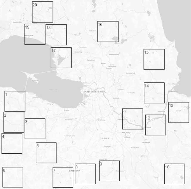
Fig. 3. Locations of the downloading squares. The numbers in the squares correspond to the index of coordinates in Table 2

Tab. 2. Coordinates of square areas of obtaining images (the latitude and longitude coordinates of the lower left corner of the square and the upper right corner of the square are indicated)

№	Coordinates of lower left corner	Coordinates of upper right corner
1.	(59.8465,29.4880)	(59.9407,29.6753)
2.	(59.7497,29.4787)	(59.8439,29.6655)
3.	(59.7194,29.6724)	(59.8136,29.8590)
4.	(59.6514,29.4612)	(59.7456,29.6474)
5.	(59.6073,29.7769)	(59.7015,29.9629)
6.	(59.4936,29.4698)	(59.5878,29.6551)
7.	(59.4928,29.9309)	(59.5870,30.1162)
8.	(59.5089,30.1352)	(59.6031,30.3206)
9.	(59.5225,30.3591)	(59.6167,30.5446)
10.	(59.5092,30.9581)	(59.6034,31.1435)
11.	(59.7649,30.5708)	(59.8591,30.7576)
12.	(59.7370,30.7824)	(59.8312,30.9691)
13.	(59.7947,30.9951)	(59.8889,31.1821)
14.	(59.8858,30.7698)	(59.9800,30.9573)
15.	(60.0399,30.7677)	(60.1341,30.9561)
16.	(60.1677,30.3435)	(60.2619,30.5326)
17.	(60.0476,29.9129)	(60.1418,30.1013)
18.	(60.1533,29.8667)	(60.2475,30.0557)
19.	(60.1550,29.6710)	(60.2492,29.8601)
20.	(60.2569,29.7411)	(60.3511,29.9307)

3. Results

The results of OSM objects manual mapping into the developed classification of the applicable surfaces for seismic modules installation have shown no collisions and mistakes in classes labels. The general numerical pa- rameters of the dataset are presented in Table 3. Table 4 represents statistics for each class of surfaces considering for seismic modules installation. In order to show the need of thorough manual inspection of OSM objects, we present in Table 4 the number of OSM classes that correspond to each class of surfaces considering for seismic module installation. That number was obtained by manual inspection of the distinct OSM objects.

Tab. 3. Overall dataset statistics

Dataset parameter	Parameters value
Number of survey dates	10
Number of geographic locations	20
Total number of images	200
Image size, px	(1050 × 1050)
Number of spectral bands	13
Number of classes	9
Total area, km2	2205
Total labelled area, km2	2002
Portion of labelled area, %	90

4. Discussion

The detailed manual inspection of the distinct OSM objects has shown its effectiveness: the mapping from OSM classes into the developed classification have passed without errors and collisions in classes of surfaces considering for seismic modules installation. On the other hand, the inspection process require thorough inspection of each object placed on the area of interest. However, it is an involuntary decision caused by the impossibility of direct mapping all the OSM classes to the developed classification of the surfaces that are applicable for the seismic sensors installation. The number of the OSM classes corresponding to some classes of seismic modules surfaces (e.g., class “Bulidings” correspond to 282 different OSM classes) confirms the need of thorough manual inspection of OSM objects classes (Table 4).

Another interesting result is the coverage of the OSM classes segments. The obtained labels cover 90% of the image areas that justifies that GIS data is suitable for satellite imagery labelling (especially in the case of 10/pix. spatial resolution). The class imbalance as well as classes segments intersection are the result of processing absence in order to evaluate raw OSM labeling segments.

Tab. 4. Statistics of each class

Class name	Total area, km2	Portion of labeled, %	Number        of objects	Number of corresponding OSM classes
Applicable Forest	1137.5	51.6	4347	7
Non-applicable Forest	34.3	1.6	252	4
Applicable Ground	1.3	0.0	105	5
Non-applicable Ground	11.6	0.1	85	12
Applicable Low Bushes	112.3	5.1	2240	21
Non-applicable Low Bushes	72.9	3.3	959	31
Applicable Wetlands	177.1	8.0	652	2
Non-applicable Wetlands	11.2	0.1	328	4
Buildings	219.9	10.0	87369	282
Transport Infrastructure	106.9	4.9	24450	41
Water	117.6	5.3	2895	21

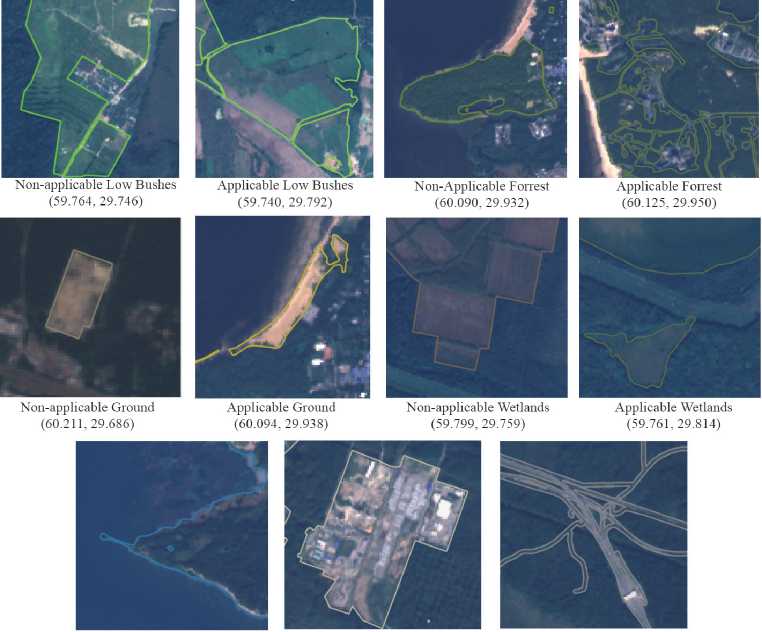
Water                            Buildings                          Transport

(60.069,29.936)                   (60.136,30.017)                   (60.134,30.062)

Fig. 4. Labelling using Sentinel-2 L2A Images using OSM data. Each of 11 classes of surfaces is shown accompanied by the corresponding coordinates

Fig. 4 presents the instances of segmentation masks.

Conclusion

The developed methodology provides obtaining large datasets of satellite images. The geospatial images in the datasets meets the necessary conditions: geographic variability, multiple time stamps, forming images under the same lighting conditions. These conditions provides representativeness of the data. The developed classification of applicable surfaces for seismic modules installation as well mapping procedure from OSM classes to the developed class hierarchy provides the relevance of the data. In addition, the mapping procedure ensures the absence of collision and mistakes in the resulting labelling. Further, we plan to assess the accuracy of OSM georeference and perform geospatial labelling over time in order to obtain proper georefernces for the images obtained at different times. The proper labelling, in turn, paves the way to the proper analysis of the features of the images.

The future work will be devoted to another issues of mistakes in georeferences of the OSM objects, training and testing machine learning models on the labelled dataset.

Acknowledgments

The study was supported by the Russian Science Foundation grant No. 22-69-00231,