A New Algorithm for Computationally Efficient Modified Dual Tree Complex Wavelet Transform

Автор: SK.Umar Faruq, K.V.Ramanaiah, K.Soundara Rajan

Журнал: International Journal of Image, Graphics and Signal Processing(IJIGSP) @ijigsp

Статья в выпуске: 7 vol.6, 2014 года.

Бесплатный доступ

We introduce a new generation functionally distinct redundant free Modified Dual Tree Complex Wavelet structure with improved orthogonality and symmetry properties. Traditional Dual Tree Complex Wavelets Transform (DTCWT), which incorporates two operationally similar, procedurally different Discrete Wavelet Transform (DWT) trees, is inherently redundant and computationally complex. In this paper, we propose Symmetrically Modified DTCWT (SMDTCWT) to explore the close relationships between the wavelet coefficients from the real and imaginary tree of the dual-tree CWT with an advent of a Quadrature Filter. This exploitation can reduce the level of redundancy that currently exists in a dual-tree wavelet system and decrease the computational complexity .Some of the primary constraints include that the designed algorithm should be satisfying the Hilbert transform pair condition and should have high coding gain, good directional sensitivity, and sufficient degree of regularity.

Еще

DWT, DTCWT, MDTCWT, Hilbert transform, Quadrature filter, computational complexity

Короткий адрес: https://sciup.org/15013364

IDR: 15013364

Текст научной статьи A New Algorithm for Computationally Efficient Modified Dual Tree Complex Wavelet Transform

Published Online June 2014 in MECS DOI: 10.5815/ijigsp.2014.07.06

A clear introduction of the DTCWT was made in [1] [2], and showed which has desirable properties of approximate shift insensitive and good directionality. These properties will play a key role for many applications in image analysis and synthesis, like denoising, deblurring , super-resolution, watermarking[3], segmentation[4] and pattern classification[5].Traditional DWT can only exhibits the shift independence in its undecimated form, which is computationally inefficient, particularly in multiple dimensions. The directional selectivity of the DWT is poor because the separability cannot distinguish between the edge and ridge features on opposing diagonals. With conventional approach, to get optimal shift independence, mid-way location of the scaling basis functions of imaginary tree between those for real tree at each level of the transform is must and it was proposed achieving this by a delay of one sample between the same level filters in each tree, and then, for subsequent levels, by employing alternate odd and even length linear-phase filters. In [6], Nick Kingsbury proposed a new approach to achieve optimal shift invariance [7] with only even length linear phase filters by highlighting the major limitations of the alternate even and odd length filter approach. The limitations of the alternate odd and even length filter approach are 1) The sub-sampling structure is not very symmetrical 2) The two trees have a slightly different frequency responses and 3) The filter sets must be bi-orthogonal. To overcome all of the above limitations, Kings bury proposed a Q-shift dual tree, in which the filters beyond the level 1 are even length, but they are no longer strictly linear phase and offers a group delay of quarter sample. But there are certain drawbacks are inherent in the above approach proposed by the Kingsbury .The most important of those are a) Even though with an employment of even length filter from second level onwards there will be a process non homogeneity between the first and the other subsequent levels due to filter mismatch b) Irrespective of the length type of the filter, equal number of separate filters employed for both real and imaginary trees. c) Filter count increases to twice as that of DWT d) Due to increased filter count the process load and computational complexity increases Considerably.

In order to reduce the process complexity and to considerably speed up the process, we proposed a modified version of the DTCWT which reduces the filter count to half to that of the conventional DTCWT (CDTCWT).The Modified DTCWT (MDTCWT) processes the signal in only one tree and obtains the equivalent other tree with an advent of Quadrature filter. All the filters used here are the same even length filters which accordingly avoids the process in homogeneity in sub sequent levels. As the filter count and designing complexity decreases, the computational complexity of the MDTCWT reduces considerabl.

II. Design method

The CDTCWT generally deploys two separate decomposition trees among which one tree is considered to be as real tree and other is considered to be as imaginary tree.(fig.1).The real decomposition tree employs a low pass filter LiO-y ( n ) and a high pass filter Hi_r (n) , in a similar manner the imaginary tree also consists of a low pass filter Lo_t (n) and a high pass filter Hit (n) .The filter pair in real tree differs with that in an imaginary tree by half sample delay, there by satisfying the Hilbert transform condition[8].

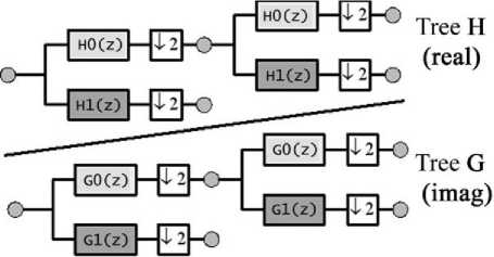
Fig 1. Kingsbury’s dual-tree CWT.

In General the filtering operation is essentially a convolution of filters impulse response h (n) and input signal x(n).A convolution is a sequence of multiplications, additions and shifting operations. Although the time required for one addition and one shifting operations is less, the time needed for one multiplication operation is considerably high(according to booths multiplication algorithm).This process time is very large compared to that required for a single addition and shift operation. If suppose for an input signal X of length ‘ m’ , a total of m convolution (L*m-1 addition, L*m multiplication and shift) operations are required. Hence, a filtering operation has to perform the convolution operations in a large number. Such an implementation demands both large number of computations and large storage features that are not desirable for either high speed or low power applications. In order to reduce the process complexity and amount of hardware, instead of implementing the imaginary decomposition tree with a dedicated low pass and high pass filter pair, we propose to derive the imaginary tree from the real tree using Quadrature Filter (QF). It can be implemented with a few shifting and Fourier conjugation operations (which will consume a negligibly very less process time) leads toget rid of the separate filter pair for analysis and synthesis of the imaginary tree and hence the decomposition in an imaginary tree is removed. This will not only leads to the reduction of the computational complexity and power consumption, but also it greatly reduces the computation time and power consumption.

Thus, a CDTCWT is suitably modified to yield a computationally efficient faster decomposition process, with the same protocol structure. The MDTCWT also employs an approximately shift invariant, directional selective dyadic decomposition tree features as that of the CDTCWT, but with single tree processing. Thus, the MDTCWT offers dual tree benefits with single tree processing. As the output of the QF is equivalent to that would be obtained with separate decomposition with Hilbert filter pair, the imaginary tree obtained with quadtrature filter will also form a Hilbert transform pair with real tree coefficients which are given as an input to the QF.This fact is true, both for theoretical and practical analysis. In CDTCWT, the Hilbert relation between the in-phase (real) and quadrature (imaginary)trees are,

Go (w)≃ H_Q (w)×e ^je ( ) _, e (w)= (1)

Gi (w)≃ Hi (w)×e ^{76 (} , e (w)= (2)

Where (jQ and ^1 are low pass and high pass filters in imaginary tree, ^0 and ^1 are filter pair in real tree.

The above equations reveals the fact that, the low pass and high pass filters in imaginary tree are related to those in real tree through Hilbert relations .The same will also be perfectly hold by the Modified DTCWT as follows.

Go (w)≃ H_o (w)×e ^{76 ( )} =QF ( H_o (w)) , 0(w)=w/2 (3)

Gi (w)≃ Hi (w)× e"^j6 ^{( )} =QF ( Hi (w)) , 0(w)= (4)

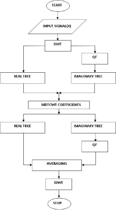
III. Algorithm structure

The following list summarizes the steps in the proposed QF Algorithm

1. Let X_T be the real tree coefficient matrix of the input signal X(m,n) and shift the x_r
2. Compute N-point FFT of the result produced in step 1.
3. From an appended zero matrix h of size N proportional to the non-empty input signal matrix X, if N is non zero integer and twice the fixed value of half of N, then make h [1 ] =1and h[2:
4. Now take the proper product of the dimensionally shifted input X_r and zero appended matrix h and compute the inverse FFT of the result.
5. shift the result produced in step.4 dimensionally in reverse approach to that in Step.1 to include the removed leading singletons.
6. The result is the quadratic ally shifted version (analytic signal) of the input. To prove the filter’s functionality practically, let as shown in table (1). Now discrete wavelet decomposition will be performed on.

Dimensionally by N( where N value is based on the size of the input X) and leading singleton dimensions are removed.

]=2,

Table 1.The stepwise operational results of the QF algorithm.

Operational Step	Operational Results
Input(X)	[ 55 127 68 178 ; 196 202 245		213 ; 223 252 117 123 ; 156 197 193	143]
Xr	208.2500 326.0654 364.5000 -048.0644 -025.0992 -032.9090	235.4702 336.2500 -107.8202 -101.6420 343.2117 374.2947 082.8729 065.7227 397.2104 294.0000 -055.4256 -039.1429 -057.4772 064.5189 -024.7500 -058.8503 -019.0724 020.9264 003.7997 -051.4306 013.1679 -031.1769 -004.5000 045.8755		-61.0548 -60.0700 29.4449 53.2500 13.5364 -21.0000
Step 1	Xrs = 208.2500 326.0654 364.5000 -048.0644 -025.0992 -032.9090	235.4702 336.2500 -107.8202 -101.6420 343.2117 374.2947 082.8729 065.7227 397.2104 294.0000 -055.4256 -039.1429 -057.4772 064.5189 -024.7500 -058.8503 -019.0724 020.9264 003.7997 -051.4306 013.1679 -031.1769 -004.5000 045.8755		-61.0548 -60.0700 29.4449 53.2500 13.5364 -21.0000
Step 2	N-point FFT(Xnpoint) of Xrs is 792.7 912.5 1058.8 -105.8 -139.5 233.2 – 648.3i 282.1 -646.3i 0285.8 – 587.6i -018.1 – 24.4i 058.3 – -156.1 + 26.5i -189.3 + 74.7i 0071.7 – 114.7i -145.9 -127.0i 302.6 314.7 0243.5 -213.1 -245 -156.1 - 26.5i -189.3 -74.7i 0071.7 + 114.7i -145.9 +127i 233.2 + 648.3i 282.1 + 646.3i 0285.8 + 587.6i -018.1 + 24.4i			-045.9 27.8i -176.3 +20.1i -171. - 6.5i 011.2 + 47.6i 009.7 -171 + 6.5i 011.2 – 47.6i 058.3 + 27.8i -176.3 – 20.1i
Step 3	h=[0 0 0 0 0 0],	h=[1 2 2 1 0 0];else h=[1 2 2 0 0 0];
Step 4	Xinpoint= 208.25 – 207.25i 326.07 – 90.21i 364.50 + 216.00i -048.06 + 224.94i -025.10 _ 8.75i -032.91 – 134.72i	235.47 – 190.55i 343.21 – 93.38i 397.21 + 231.34i -057.48 + 240.34i - 019.07 – 40.79i 013.17 – 146.96i	336.25 – 234.10i -107.82 – 50.44i -101.64 – 11.46i -61.05 + 22.56i 374.29 + 24.39i 082.87 – 30.25i 065.72 -36.08i -60.07 – 52.25i 294.00 + 178.85i -055.43 + 62.14i -039.14 + 71.92i 29.44 -65.43i 064.52 +157.66i -024.75 - 34.19i -058.85 +7.09i 53.25 +9.18i 020.93 + 55.25i 003.80 - 11.69i -051.43 - 60.46i 13.54 + 42.87i -031.18 – 182.05i -004.50 + 64.44i 045.88 + 28.99i 21.00 + 43.07i
Step 5	Xirs= 208.25 – 207.25i 326.07 – 90.21i 364.50 + 216.00i -048.06 +224.94i -025.10 - 8.75i -032.91 – 134.72i	235.47 – 190.55i 343.21 – 93.38i 397.21 + 231.34i - 057.48 +240.34i - 019.07 – 40.79i 013.17 – 146.96i	336.25 – 234.10i -107.82 – 50.44 -101.64 –11.46i 374.29 + 24.39i 082.87 – 30.25i 065.72 - 36.08i 294.00 + 178.85i -055.43 + 62.14i -039.14 +71.92i 064.52 +157.66 -024.75 - 34.19i -058.85+7.09i 53.25 020.93 + 55.25i 003.80 - 11.69i -051.43 - 60.46i -031.18 – 182.05i -004.50+ 64.44i 045.88 + 28.99i		-61.05 + 22.56i -60.07 – 52.25i 29.44 -65.43i +9.18i 13.54 + 42.87i -21.00 + 43.07i
Step 6	The analytic signal 208.25 – 207.25i 326.07 – 90.21i 364.50 + 216.00i -048.06 + 224.94i -025.10 - 8.75i -032.91 – 134.72i	for the given input signal is= 235.47 – 190.55i 336.25 – 234.10i -107.82 – 50.44i -101.64 – 11.46i 343.21 – 93.38i 374.29 + 24.39i 082.87 – 30.25i 065.72 -36.08i 397.21 + 231.34i 294.00 + 178.85i -055.43 +62.14i -039.14 +71.92i -057.48 + 240.34i 064.52 + 157.66i -024.75 -34.19i -058.85 +7.09i 53.25 -019.07 – 40.79i 020.93 + 55.25i 003.80 -11.69i -051.43 -60.46i 013.17 – 146.96i -031.18 – 182.05i -004.50 + 64.44i 045.88 + 28.99i			-61.05 + 22.56i -60.07 – 52.25i 29.44 -65.43i +9.18i 13.54 + 42.87i -21.00 + 43.07i

The realizable approach of the Modified DTCWT does not contain the filters Go and ^1 ,rather it implements the functionality of (jQ as QF(Hq ) and ^1 as QF(Hi).All the conditions imposed in CDTCWT by the Hilbert relations cited above are greatly abide by the Modified DTCWT ,with the completely excluded filter pair GQ and Gi .The resultant coefficients of wavelet decomposition in imaginary tree if it could have been performed with filters Gq and G^ ,can easily be obtained in the Modified DTCWT with a simple quadrature filter ,which is faster,flexible, in operation and has compact hard ware, instead of performing the decomposition with the filter pair (jQ and ^1 .The process inside the Modified DTCWT is illustrated in fig(2).

In poly phase notation [9], the transfer functions of the filters used for real tree decomposition can be written in terms of their even and odd phases according to the following relations. The filter pair used here is represented in poly phase notation as follows.

For analysis

Ho (z) = H Az2 )+z -iHo Az2)(5)

Hi (z)=Hi Az2 ) + z ~1 Hi Az2)(6)

for synthesis

Fo (z) = F00(z2 )+z~ 'Fo ((z 2 )

F. (z)=Fi Az 2 ) + z~1 Fi i(z 2 )

Hi (n) = (-1)"Ho(L-n-1)(9)

Fi (n) = (-1)"Fo(£-n-1)(10)

And the high pass filters are alternate time reversals of the low pass filters.

Hi (n) = (-1)nHo(L-n-1)(11)

Fi (n) = (-1)”Fo(L-n-1)(12)

Where L is length of the filters.

The impulse response of the low pass and high pass filter pair used for analysis and synthesis of real tree are plotted in figure (3).

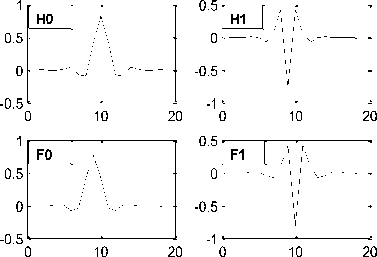
Fig (3):Impulse responses of the analysis and synthesis filter pairs of the real tree with a selected wavelet type of ‘bior6.8’.

The filter coefficients for both analysis and Synthesis real tree filters are listed in table(2).

Table (2): Coefficients for analysis and synthesis filter pairs

H0	H1	F0	F1
0	0	0	0
0.0019	0	0	-0.0019
-0.0019	0	0	-0.0019
-0.0170	0.0144	0.0144	0.0170
0.0119	-0.0145	0.0145	0.0119
0.0497	-0.0787	-0.0787	-0.0497
-0.0773	0.0404	-0.0404	-0.0773
-0.0941	0.4178	0.4178	0.0941
0.4208	-0.7589	0.7589	0.4208
0.8259	0.4178	0.4178	-0.8259
0.4208	0.0404	-0.0404	0.4208
-0.0941	-0.0787	-0.0787	0.0941
-0.0773	-0.0145	0.0145	-0.0773
0.0497	0.0144	0.0144	-0.0497
0.0119	0	0	0.0119
-0.0170	0	0	0.0170
-0.0019	0	0	-0.0019
0.0019	0	0	-0.0019

The decomposition process in the traditional DTCWT and Modified DTWCT are absolutely similar in all aspects. The signal decomposition in first level with the MDTCWT and the CDTCWT are practically verified and summarized in table (3).

Table (3): Simulation results of an example signal(x(m,n))wavelet decomposition using the CDTCWT and MDTCWT with a Daubechies second wavelet ‘db2’.

v Level 1 real tree operation with CDTCWT		Level 1 imaginary tree operation with CDTCWT
Original input (X(m,n)	55 127 68 178 196 202 245 213 223 252 117 123 156 197 193 143	Original input (X(m,n)	55 127 68 178 196 202 245 213 223 252 117 123 156 197 193 143
Ca1	208.2500 235.4702 336.2500 326.0654 343.2117 374.2947 364.5000 397.2104 294.0000	Ca2	208.25 – 207.25i 235.47 – 190.55i 336.25 – 234.10i 326.07 – 90.21i 343.21 – 93.38i 374.29 + 24.39i 364.50 + 216.00i 397.21 + 231.34i 294.00 + 178.85i
Ch1	-107.8202 -101.6420 -061.0548 082.8729 065.7227 -060.0700 -055.4256 - 039. 1429 029.4449	Ch2	-107.82 – 50.44i -101.64 – 11.46i -61.05 + 22.56i 082.87– 30.25i 065.72 - 36.08i -60.07 – 52.25i -055.43 + 62.14i -039.14 + 71.92i 29.44 - 65.43i
Cv1	-048.0644 - 057.4772 064.5189 -025.0992 - 019.0724 020.9264 -032.9090 013.1679 - 0311769	Cv2	-48.06 + 224.94i -57.48 + 240.34i 64.52 + 157.66i -25.10 - 8.75i -19.07 – 40.79i 20.93 + 55.25i -32.91 – 134.72i 13.17 – 146.96i -31.18 – 182.05i
Cd1	-024.750 -58.8503 53.2500 003.799 -51.4306 13.5364 -004.500 45.8755 -21.0000	Cd2	-24.7500 - 4.7918i -58.8503+56.1797i 53.2500-19.9396i 03.7997-11.6913i -51.4306-60.4635i 13.5364 +42.8683i - 04.5000+16.4832i 45.8755+ 4.2838i -21.0000 -22.9287i
Level 1 real tree operation with MDTCWT		Level 1 imaginary tree operation with MDTCWT
Ca1	208.2500 235.4702 336.2500 326.0654 343.2117 374.2947 364.5000 397.2104 294.0000	Ca3	208.25 – 207.25i 235.47 – 190.55i 336.25 – 234.10i 326.07 – 90.21i 343.21 – 93.38i 374.29 + 24.39i 364.50 + 216.00i 397.21 + 231.34i 294.00 + 178.85i
Ch1	-107.8202 -101.6420 -61.0548 082.8729 065.7227 -60.0700 -055.4256 -039.1429 29.4449	Ch3	208.25 – 207.25i 235.47 – 190.55i 336.25 – 234.10i 326.07 – 90.21i 343.21 – 93.38i 374.29 + 24.39i 364.50 + 216.00i 397.21 + 231.34i 294.00 + 178.85i
Cv1	-48.0644 -57.47720 64.5189 -25.0992 -19.07240 20.9264 -32.9090 13.16790 -31.1769	Cv3	-48.06 + 224.94i -57.48 + 240.34i 64.52 + 157.66i -25.10 - 8.75i -19.07 – 40.79i 20.93 + 55.25i -32.91 – 134.72i 13.17 – 146.96i -31.18 – 182.05i
Cd1	-24.7500 -58.8503 53.2500 03.7997 -51.4306 13.5364 -04.5000 45.8755 -21.0000	Cd3	-24.7500 - 4.7918i -58.8503+56.1797i 53.2500-9.9396i 03.7997-11.6913i -51.4306-60.4635i 1 03.5364 42.8683i -04.5000+16.4832i 45.8755+ 4.2838i -21.0000 -22.9287i

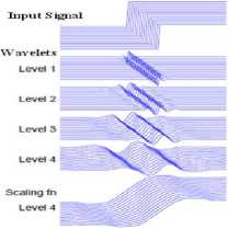
The shift sensitive characteristics of the MDTCWT are similar to that of the CDTCWT and still even flat step response is possible with the MDTCWT. The shift sensitive characteristics of the MDTCWT are psycho– visually similar to those can be obtained with the CDTCWT. In the MDTCWT as the levels of decomposition increases, the step wavelet response will get even flat and smoother. For example a composite signal of 16 shifted step functions are applied as an input to both modified MDTCWT and standard DWT simultaneously to observe the variation in shift insensitivity offered by them at levels from 1 to 4 as shown in figure (4) and has been observed that the characteristics are alike in all aspects to those can be obtained with CDTCWT but relatively very less shift effects. There is almost no change in shape of the step response and the shifted wavelet response will remains as same as that of the un-shifted step response. Hence as the levels of decomposition increases, the deviation between the shifted and the non-shifted waveforms vanishes proportionally with the MDTCWT as shown in figure (4).

MDTCW7

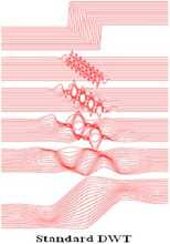
f igure (4):s hift -invariance characteristics of the MDTCWT.

The Multi scale analysis is an important feature offered by the Conventional DTCWT, according to which as the scale or level of decomposition increases the regularization in time and frequency domains will get improved. Signal decomposition at lower scales or levels ,it is only poor fair timefrequency resolution is possible, but as we progress the decomposition process to the higher scales or higher levels it is possible to obtain better, desirable resolution in time and frequency domains. But when the levels or scales of decomposition are increased beyond certain value the quality of reconstructed signal will decreases in the Conventional DTCWT. Hence the quality of the reconstructed signal will limit the levels of decomposition in the Conventional DTCWT. But the MDTCWT is completely impervious to this problem, and can allow the decomposition at any higher level without a significant information loss. Multilevel wavelet decomposition structure is illustrated in figure(5) The scale by scale wavelet coefficients of an example signal(x(m,n)) decomposition in real and imaginary trees are summarized in table(4) and table(5) respectively.

LL³	LH³	LH²	LH¹
HL³	HH³
HL²		HH²
HL¹			HH¹

Fig(5):Multi-scale decomposition structure of the Modified DTCWT

Since in CDTCWT, the decomposition process occurs in two separate trees, the significant amount of information loss occurs during the process of retaining the higher coefficient values and removes the lower coefficient values. The same process will continue as the decomposition progresses to the higher levels .To explain how the CDTCWT generates oriented wavelets ,let us now consider the 2-D wavelet ф (x, у) = р(х)р(у) associated with the row column implementation of the wavelet transform ,where (to is a complex(approximately analytic)wavelet given by ф (x) = рh (x) + jгрд (x) -We obtain for Ф(x,у) the expression гр(x, у) = [гр h (x) + j ФаМ^^У) + j (уСУ)] = Ф1гМФ/гМ - фдМФдМ + j[Фg(X)гp((у) +

Фп МФдМ (13)

Note that the first term in above equation гр _h (x)p_h (y) is HH wavelet of a real tree wavelet decomposition.The second term ф_д (х)Ф_д (у) is also a HH wavelet associated with the imaginary tree wavelet decomposition. For instance, to obtain a real 2-D wavelet oriented at +45⁰, consider now the complex 2-D wavelet гр₂(,х,у) = гр (х)р(у) ,where р(у) represents the complex conjugate of Ф(to and ,as previous, р(х) is approximately analytic wavelet р(х) = гр _h(x) + j Ф_g(x) .We obtain for

( , ) the expression ф2 (x, у) = [гр h(x) +j (gto^phCy) + ppg(y()

= [р h⁽x) + jФg⁽X⁾][ф (⁽у) -j^gto]

= ФxtoФуto + ФдМ)Фд(У)

+ j [р д to^h to — Фк to^g to (14)

To obtain four more oriented real 2-D wavelets, we can repeat this procedure on the following complex 2-D wavelets ф(x) ((у) , ф (у) р(x) , ф (x) ( (у) and p(^y) (to ,where гр (х) = гр _h (х) + j гр _g(x) and

ф(x) = ф(to) + jФ_д (x).Specifically, we obtain the six wavelets using the following equations.

грt Му) = ^=(Ф i ,^ x,у) - гр₂,t ⁽x, у) (15)

(i + з ^.у) = ^=(Ф i ,^ x,у) - гр ₂,t ⁽x, у) (16)

For i=1, 2, 3, where the two seperable 2-D wavelet bases are defined in the usual manner;

(1 , 1 ⁽x , у) = ф (to( ⁽(у)р Ф 2, 1 ⁽x , у) = Ф д ⁽Х)Р д ⁽У),

(1 ,2 ⁽x, у) = ф(to( 11 to , Ф2,2 ⁽x, у) = Ф д ⁽у)р д ⁽х),

Ф 1 ,3 ⁽x , у) = Ф (МФ ((У), Ф 2,3 ⁽x , У) = Фд(х)Фд(),'),

We have used the normalization 1/(2 only so that the sum/difference operation constitutes an orthonormal operation.

The CDTCWT can provide good directional selectivity in only six orientation angles viz ±150,±450 and ±750 while preserving the quality of reconstructed signal. The directional wavelet orientation of the MDTCWT is shown in fig (6).In order to further increase the chances of wavelet orientation in even more directions, the levels of signal decomposition has to be brought to the higher scales. If this happens a huge amount of significant information will be lost in both the trees of CDTCWT, while discarding the smaller coefficients. This will leads to the remarkable drop in the quality of the reconstructed signal. Hence the directional wavelet orientation and levels of decomposition are limited by the reconstructed signal quality. But with Modified DTCWT the case is entirely different. While providing the directional wavelet orientation in all six angles as that of the CDTCWT, it does not limit the chances of wavelet orientation in even more directions and levels of decomposition with the reconstructed signal quality. A most convincing reason for this is the Modified DTCWT performs the signal decomposition in only one tree and maintains a perfect information integrity which does not allow any significant information loss. Hence if we brought the decomposition to higher scales we can achieve the better wavelet orientation in even more irections without losing the quality of the reconstructed signal.

Table(4) Multiscale wavelet coefficients for real tree decomposition of the example input signal(X(m,n)).

Scale or Level

Ca1

Ch1

Cv1

Cd1

Scale 1

208.2500 235.4702 336.2500

326.0654 343.2117 374.2947

364.5000 397.2104 294.0000

-107.8202 -101.6420 -

61.0548

082.8729 065.7227 -

60.0700

-055.4256 -039.1429

29.4449

-48.0644 -57.4772

64.5189 -25.0992 -19.0724

20.9264 -32.9090 13.1679 -

31.1769

-24.7500 -58.8503

53.2500 03.7997 -51.4306

13.5364

-04.5000 45.8755

-21.0000

Scale

487.7586 519.1071 684.8755

587.6252 611.4440 709.6574

760.7854 772.4277 624.8238

-99.8501 -92.2430 -

36.1927

42.2636 39.3370 -

27.2889

57.5864 52.9060

63.4815

-21.3923 46.1985 -

24.8062

-18.7314 26.9029 -

8.17150

-26.6268 -44.6692 71.2960

-3.7777 15.8881

-12.1104

-2.5714 -19.4321

22.0035

6.3491 03.5440

- 09.8931

Scale

1040.2 1084.2 1367.6

1143.0 1178.0 1381.7

1522.5 1513.8 1286.1

- 084.8568 -78.2740 -

24.7841

102.9904 90.8790 -

29.5031

-018.1336 -12.6050

54.2872

-25.5184 79.8325 -

54.3141

-22.1482 57.0891 -

34.9409

-10.1922 -66.5056

76.6978

-2.8237 15.2228

-12.3991

3.2330 -34.5012

31.2682

-0.4093 19.2784

-18.8691

Table(5): Multiscale wavelet coefficients for imaginary tree decomposition of the example input signal(X(m,n))

Scale or Level	Approximate and Horizontal coefficients		Vertical and Detail coefficients
Scale 1	Ca2	208.25 + 22.19i 235.47 + 31.18i 336.25 -46.36i 326.07 – 90.21i 343.21 – 93.38i 374.29 +24.39i 364.50 + 68.02i 397.21+ 62.20i 294.00+ 21.97i	Cv2	-48.0644 - 4.5090i -57.4772 +18.6140i 64.5189 - 30.0819i -25.0992 - 8.7500i -19.0724 -40.7870i 20.9264 +55.2500i -32.9090 +13.2590i 13.1679 +22.1730i - 31.1769 - 25.1681i
Scale 1	Ch2	-107.82- 79.85i -101.64 – 60.54i -61.05 + 51.68i 082.87- 30.25i 065.72 – 36.08i -60.07 – 52.25i -055.43 + 110.10i -039.14 + 96.63i 29.44 +00.57i	Cd2	-24.7500 - 4.7918i -58.8503 +56.1797i 53.2500 - 19.9396i 03.7997 -11.6913i -51.4306 -60.4635i 13.5364 +42.8683i -04.5000 +16.4832i 45.8755 + 4.2838i -21.0000 - 22.9287i
Scale 2	Ca2	487.76 + 99.97i 519.11 + 92.94i 684.88 -48.98i 587.63 – 157.63i 611.44 – 146.25i 709.66 + 34.67i 760.79 +57.66i 772.43 +53.31i 624.82 + 14.31i	Cv2	-21.3923 - 4.5584i 46.1985 -41.3222i -24.8062 +45.8805i - 18.7314 + 3.0221i 26.9029 +52.4625i -08.1715 -55.4846i - 26.6268 + 1.5363i - 44.6692 -11.1403i 71.2960 + 9.6041i
Scale 2	Ch2	-99.85 + 8.84i -92.243+ 7.8341i -36.1927 +52.4063i 42.2636 -90.896i 39.337 -83.80i -27.2889 - 57.5469i 57.5864 +82.04i 52.906 +75.967i 63.4815 + 5.1406i	Cd2	- 3.7777 + 5.1503i 15.8881 +13.2653i -12.1104 - 18.4155i - 2.5714 - 5.8467i -19.4321 + 7.1269i 22.0035 - 1.2802i 6.3491+0.6965i 03.5440 -20.3922i -09.8931 +19.6957i
Scale 3	Ca2	1040.2 +219.1i 1084.2 +193.9i 1367.6 -055.2i 1143.0 -278.5i 1178-248i 1381.7 + 047i 1522.5 +059.4i 1513.8 +054.1i 1286.1+008.1i	Cv2	- 25.5184 + 6.9028i 79.8325 -71.3574i -54.3141 +64.4546i - 22.1482 - 8.8486i 57.0891 +84.4884i -34.9409 - 75.6398i - 10.1922 + 1.9458i - 66.5056 -13.1309i 76.6978 +11.1852i
Scale 3	Ch2	-084.86-69.93i -78.27 -59.75i -24.78 + 48.38i 102.99 -38.52i 90.88 -37.91i -29.50 -45.65i -181.3 + 108.45i -12.60 +97.66i 54.29-02.72i	Cd2	- 2.8237 - 2.1029i 15.2228 +31.0497i -12.3991 - 28.9468i 3.2330-1.3939i -34.5012 - 2.3415i 31.2682 + 3.7354i - 0.4093 + 3.4968i 19.2784 -28.7082i -18.8691 +25.2114i

(a) REAL TREE

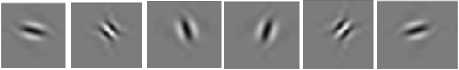
-15° -45° -75° 15° 45° 75 °

(b) IMAGINARY TREE

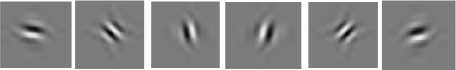
-15° -45° -75° 15° 45° 75 °

■ИНН

-15° -45 ° -75° 15° 45° 75 °

Fig(6):Directional wavelet orientation of the MDTCWT, that are obtained with,(a)real tree (b)imaginary tree and (c)magnitudes of dual tree complex wavelets

IV. Computational complexity

In past DTCWT approaches and in Kingsbury’s approach the transform makes use of two DWT trees. Each tree will have a pair of low pass and high pass filters. Let in Kingsbury approach, [LоDT (n), HiDr(n)} be the filter pair for real tree, with transfer functions [LоDr (z), HiDr(z)] . In a similar manner [LоОг(п),ЯiDj(n)} is the filter pair for the imaginary tree with functions[LoDi (z), HiD;(z)}.

Fro[10] the number of complex computations insteadobtaining it directly from the real tree with neededfor CDTCWT is investigated analytically and compared with that needed for MDTCWT. For each versions individual number of operations needed are calculated for both real and imaginary trees separately and then overall computations .In case of CDTCWT for real tree a total of 2(\Я t D_r(z)\ + \L оD _r(z)\ + 1 ) complex computations are needed. Similarly for an imaginary tree a total of (| ( )| + | ( )| + ) complex computations are required. Thus on a whole the CDTCWT needed 2 (\Я ID _r(z)\ + \L о D_r(z)\ + \Я ID ;(z)| + |LoD;(z)| + 2) complex computations as in table (6). But in the case of the MDTCWT ,the total number of complex computations needed are get reduced to approximately half to that in the CDTCWT, because the imaginary tree does not involve the process QF(process involves simple shift and fourier conjugate operations,) as in table(7).Hence the MDTCWT requires only approximately (| ( )| + | ( )| + ) complex computations.

A practical verification of the computational efficiency offered by the MDTCWT is compared with the CDTCWT by taking into account the numerical value of the spectral lengths of the filter pair used for analysis in both real and imaginary trees of the respected. Thus the number of complex operations needed to process a 64X64 image can be estimated as in table (8).The computational complexity of the MDTCWT is compared through graphical illustration and it is shown in figure (7).

Table (6): complex computations for conventional DTCWT.

TCW T	Real	Imaginary	Total
Multipli cations	\H i D_r(z)\ + \L о D_r(z) \ +2	\Я iD i (z)\ + \L о D , (z)\ + 2	\HiD_r(z)\ + К oD_r(z)\ + \//iD i (z)\ + \LoD , (z)\ + 4
Additi ons	\H i D_r(z)\ + \L о D_r(z)\	\HiD_;(z)\ + \|LoD_i(z)\	^ iD_r(z)\ + \LoD_r(z)\ + \HiD_t(z)\ + \LoD_f(z)\
Total	2 (\|HiD_r(z)\| + \|LoD_r(z)\| + 1)	2 (\Я iD _i(z)\ + \£ oD _f(z)\ + 1)	2 (\|HtD_r(z)\| + \L oD_r(z)\ + \HtD _t(z)\ + \L oD _t(z)\ + 2)

Table (7): complex computations for MDTCWT

For MDTCWT	REAL	Imaginary	Total
Multiplications	\HtD_r(z)\ + \L o D_r(z) \ + 2	~< 1	\H ID _/(z)\ + \L о D _/(z)\ + 2
Additions	\|ЯiD_r(z)\| + \|LoD_r(z)\|	~< 1	\H ID _/(z)\ + \L о D_t(z)\
Total	2 (\Я iD_r(z)\ + \LoD_r(z)\ + 1)	~< 2	2 (\ЯiD_r(z)\ + \LoD_r(z)\ + 1)

Table (8): operations required for processing a 64X64 image with conventional DTCWT and modified MDTCWT.

CDTCWT				MDTCWT
Input size	64X64 image			64X64 image
Operation	Real tree	Imag Tree	DTCWT	Real tree	Imag Tree	MDTCWT
Multiplication s	155648	155648	311296	155648	< 4096	159744
Additions	147456	147456	294912	147456	< 4096	159744
Total	303104	303104	606208	303104	< 8192	319488

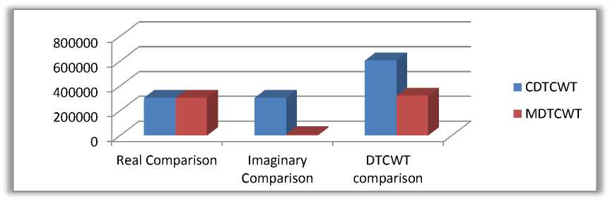
Fig (7): computational complexity between CDTCWT and MDTCWT

V. Conclusion

The MDTCWT achieves a nearly shift invariant and directionally selective properties with a redundancy factor of 1 d for‘d’- dimensional signals, and the signal of any(d)dimension will be decomposed in only one tree. For 2 dimensional signal the redundancy factor is 1 ² =1, so the entire data in the decomposed signal is significant and hence there is no redundant data.Thus the MDTCWT is completely redundant free compared to the Conventional Dual Tree Complex Wavelet Transfom. The proposed work is computationally more efficient than the CDTCWT as from the fact that, the modified MDTCWT obtains its imaginary straight away from the real and it does not requires separate tree. The tool developed is obeyed to all conditions of DTCWT integrity and preserves all the performance features.

The MDTCWT has a huge scope in the signal processing plot forms where process speed and power consumption are the major factors to be considered .It finds its applications in image analysis and synthesis, like denoising, deblurring, super-resolution, watermarking [4], segmentation [3] and pattern classification [5] where processor has to process a bulk amount of data in quicker times at relatively higher speeds with process homogeneity.

Список литературы A New Algorithm for Computationally Efficient Modified Dual Tree Complex Wavelet Transform

N G Kingsbury: "The dual-tree complex wavelet transform: a new efficient tool for image restoration and enhancement", Proc. EUSIPCO 98,Rhodes, Sept 1998, pp 319-322.
N G Kingsbury: "Shift invariant properties of the dual-tree complex wavelet transform", Pro IASSP 99, Phoenix, AZ, March 1999, paper SPTM 3.6.
P Loo and N G Kingsbury: "Digital watermarking using complex wavelets", Proc. ICIP2000,Vancouver Sept 2000.
PFC de riiva'and N G kingsbury: fassegmrenatation Using level sert curves of complexwavelet sufaces" proc ICIP2000vancouver sept 2000.
J Romberg, H Choi, R Baraniuk and N G Kingsbury: "Multiscale classification using Complex wavelets", Proc. ICIP 2000, Vancouver, Sept 2000.
NickKingsbury:"A dual-tree complex wavelet transformwith improvedorthogonality and symmetry properties".
N.G. Kingsbury, "The dual-tree complex wavelet transform: A new techniquefor shift Invariance and directional filters,"in Proc. 8th IEEE DSP Workshop Utah,Aug. 9–12, 1998, paper no. 86.
H.F. Ates and M.T. Orchard, "A nonlinear image representation in waveletdomain using Complex signals with single quadrantspectrum," in Proc. AsilomarConf. Signals, Systems, Computers, 2003vol. 2, pp.1966–1970.
P P Vaidyanathan and P-Q Hoang:"Lattice Structuresfor optimal design and robust Implementationof two-channelperfect ReconstructionQMF banks", IEEE Trans. on ASSP, Jan 1988, pp 81-94.
Ingrid Daubechies and Wim Sweldens: a tutorialon "factoring wavelettransforms into lifting steps",September1996, revised.

Еще

Статья научная