A New Approach for Texture Classification Based on Average Fuzzy Left Right Texture Unit Approach

The analysis of texture in images provides an important cue to the recognition of objects. It has been recently observed that different image objects are best characterized by different texture methods. Successful applications of texture analysis methods have been widely found in industrial, biomedical, remote sensing areas and target recognition [1]. Since there are a lot of variations among natural textures, to achieve the best performance for texture analysis or retrieval, different features should be chosen according to the characteristics of texture images. A number of texture analysis methods have been proposed over the years and it is well-recognized that they capture different texture properties of the image.

To analyze and identify textures, a number of texture analysis methods have been developed. These are autocorrelation function [2], digital transformation [3], textural edges [4], structural elements [2], spatial gray level co-occurrence probability [5], Markov random fields [6], wavelet decomposition methods [7] and so on. The most commonly used approach is the spatial gray level co-occurrence matrix that provides gray-level transition information between two gray levels [8,9]. One of the simplest statistical approaches for describing texture is to use statistical moments of the gray-level histogram of an image or region. However, measures of texture computed using only histograms suffer from the limitation that they carry no information regarding the relative position of pixels with respect to each other.

He and Wang have proposed the texture spectrum (TS) approach for texture analysis [10, 11, 12, 13] that was initially used as a texture filtering approach. The TS methodology [14, 15] has been applied to texture characterization and texture classification showing its promising discrimination performance. But a major inconvenient of this descriptor is the large range of its possible values (there are 6561) at the same time that these values are not correlated. Moreover, as images of the same underlying texture can vary significantly, textural features must be invariant to (large) image variations, and at the same time sensitive to intrinsic spatial structures that define textures.

A possible solution to aforementioned problems should be the use of fuzzy logic and fuzzy techniques. Fuzzy logic is a simple and powerful tool to mathematical formalization of ill defined concepts that usually appear at texture analysis and segmentation. On the other hand, fuzzy techniques enable more flexible classifications because elements can have a characteristic only to some degree.

Taur et al. [16] proposed a texture feature based on the fuzzified relative gray levels between pixels. The simplest unit representing a pixel is a 3-vector called Texture Vector (TV). An image block is represented by the histogram of its TV, and its texture is then characterized using a neural network classifier. Later on, Aina Barcelo et al [17] used the concept of Fuzzy Texture Spectrum (FTS), to be used as the texture feature within texture analysis process. FTS will dramatically reduce the total number of texture units to 2020. However, the high dimension of 2020 is a computational burden.

The proposed approach in this paper is based on the LRTM [18] and Original TS [10], and tries to alleviate its drawbacks and aforementioned problems. So, to retain its discriminatory power, the proposed method considers a 3×3 neighbourhood into two connected fuzzy patterns. A connected fuzzy pattern approach gives complete local micro texture information and to avoid the imprecision within the process, we make use of fuzzy logic and fuzzy techniques.

The paper is organized as follows. The concepts of texture unit, and fuzzy texture unit are given in section II. The proposed methodology is given in section III. Section IV contains experimental results and conclusions are given in section V.

II. texture unit

In a square raster digital image, each pixel is surrounded by eight neighboring pixels. The local texture information for a pixel can be extracted from a neighborhood of 3×3 pixels, which represents the smallest complete unit. A general representation of texture elements are shown in Fig.1.

elements, TU= {E 1 , E 2 , E 3 , E 4 , E 5 , E 6 , E 7 , E 8 } where E i , i=1,2,3,…,8 is denoted by the following Equation(1).

f 0 if V i < V o

Ei = ^

if V i = V 0

if V i > V 0

for: i = 1,2,....8 >

and each element E i occupies the same position as the pixel i. As each element of TU has one of the three possible values (0, 1, 2), the total number of possible TU is 3⁸= 6561. These texture units are labeled by using the Equation(2)

Ntu = ^ E i 3 ' ,    Ntu e {0,1,2,(N^8-1) }       (2)

i = 1

where NTU is the texture unit number. There is no unique way to label and order the 6561 texture units. The high range of TU number makes further process on texture classification is very complicated. To overcome this, the texture units are reduced from 0:6560 to 0:255 for classification purpose by assigning binary value 0 or 1 to each element of TU and by this the corresponding NTU ranges from 0:255 [Ph.D thesis of Dr.V.Vijayakumar].

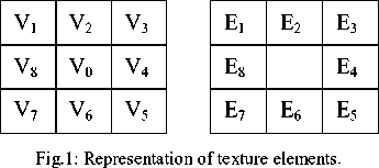
A neighborhood of 3×3 pixels can be denoted by a set containing nine elements: V= {V 0 ,V 1 ,...,V 8 }, where V 0 represents the intensity value of the central pixel and V i, where i= {1,2,….,8}, is the intensity value of the neighboring pixel i. Based on this the corresponding texture unit (TU) is defined by a set containing eight

A. Fuzzy Texture Approach

The main problem in the above two representations of TU is that they are unable to distinguish between less and far less or greater or far greater and large range of its possible values and moreover these values are not correlated. To address the above and to have high discriminating power, two more membership functions (Greater and Lesser quantities) are introduced in FTS approach. The aim of fuzzy texture unit is to extract local texture information from pixels for representing the texture accurately. To deal accurately with the regions of natural images even in the presence of noise and the different processes of caption and digitization FTS is introduced. For example, even if the human eye perceives two neighboring pixels as equal, they rarely have exactly the same intensity values. However, the desirable situation would be that the TU of homogeneous images contain more number of ones because the human eye can perceive ones. Therefore, if there is lack of ones, the basic TU will take only 0 and 2 values, which means that the real number of possible textures is 28, i.e., 256 out of 6561, and the spectrum will never be totally covered, which misuses the power of TS method.

To overcome the above, the fuzzy membership function is represented as shown in Fig.2 [19]. A texture unit is represented by eight elements each of which has only five possible values {0, 1, 2, 3 and 4} in fuzzy texture unit approach. The elements are ordered in clockwise around the centre pixel as shown in Fig.1. The following Equation (3) is used to determine the elements, E i of the texture unit. In FTU [19], the texture unit is reduced to 2020, so that the computation time is very less when compared to basic approach

• V.              V,

  ----------------------------------------------------1--------------------------------------------------------------------------------------------------------¹-------------------------------------------------------

• Vo,У,

О               4

Fig.2: Fuzzy texture number (Base-5) representation.

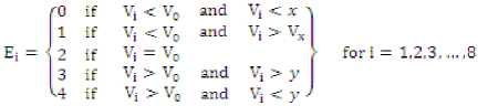
where x, y are the user-specified values.

The FTU number (FTU n ) is computed as given in Equation (4):

The FTU numbers range from 0 to 2020.

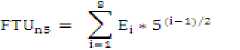
The process of evaluating FTU from a subimage of 3×3 is shown in Fig.3.

90	130	145
160	140	200
100	140	250

0	1	3
4		4
0	2	4

(a)                                   (b)

FTU= {0, 1, 3, 4, 4, 2, 0, 4}, FTU n5 = 1292

(c )

Fig.3: (a) Original subimage (b) Representation of fuzzy texture elements (c) Evaluate FTU.

• III.    proposed method fuzzy left right texture

UNIT MATRIX

The texture spectrum method of texture analysis gives the texture information using eight neighbouring pixels around the central pixel. The level of this information depends on ordering of the neighbouring pixels. Further, a little work is reported [18, 20] in literature to produce strong texture information of an image by separating the neighboring pixels into groups and form a relationship between them. In the cross diagonal approach [21, 22], texture information of the image is evaluated by separating the neighbourhood pixels into diagonal and corner pixels. The corner pixels are not connected pixels. The cross diagonal approach is evaluated with original texture unit but not with the FTU information. To overcome that, LRTM is proposed [18]. It considers the minimum of the LTUM and RTUM. By this only one of the 8 combinations of LTUM and RTUM is considered. Therefore some of the useful information will be lost by not considering the remaining 7 combinations of LTUM and RTUM. To address this proposed method considers the average of LTUM and RTUM. This results an average fuzzy left and right texture unit (AFLRTU) by the proposed scheme.

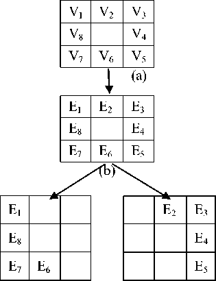
In the proposed AFLRTU method of texture analysis, the eight elements in the texture unit are obtained from a neighborhood of 3×3 pixels. They are divided into two well connected equal groups containing four pixels named as Fuzzy Left Texture Unit (FLTU) and Fuzzy Right Texture Unit (FRTU) as shown in Fig.4. This FLRTU method further reduces the FTU from 2020 to 79. This reduction is useful for a good classification by reducing computational complexity.

(c)                     (d)

Fig.4: a) Representation of a) 3×3 neighbourhood b) Texture elements c) Formation of Fuzzy left texture unit (FLTU) matrix d) Formation of Fuzzy right texture unit (FRTU) matrix.

Each fuzzy texture element in the two groups has one of the five possible values {0, 1, 2, 3 and 4} as given in Equations (5) and (6):

ⁿfltu = Ец •5⁽¹~^1,'²⁾

1=1                                                  (5)

NfRTU ^{= E}Ri * s^^1-1" ^

i=-                                                  (6)

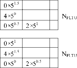
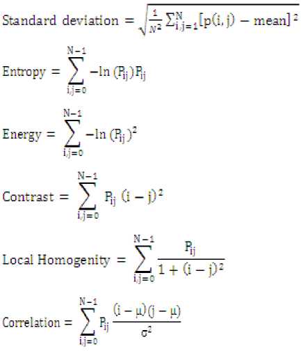
where N FLTU and N FRTU are the fuzzy left texture unit number and fuzzy right texture unit number respectively. The E Li and E Ri are the i^th element of left texture unit and right texture unit respectively. The entire process of transforming an image neighborhood into FLTU and FRTU is shown in Fig.5. The elements in the FLTU may be ordered in four different forms (i.e., (E 1 to E 6 ) or (E 8 to E 1 ) or (E 7 to E 8 ) or (E 6 to E 7 )) and FRTU may also be ordered in four different forms (i.e., (E 2 to E 5 ) or (E 3 to E 2 ) or (E 4 to E 3 ) or (E 5 to E 4 )) respectively. The values of FLTU and FRTU vary depending on the position of elements which can be labeled by using the Eqs. (5)&(6). To overcome the problem of rotational invariance in FLTU and FRTU the minimum value of FLTU and FRTU is considered as the final FLTU and FRTU. Based on this the uniform FLTU and FRTU values of Fig.5 are the min(31,  14, 49, 22) and min(72, 43, 52, 66)

respectively.

0
4
0	2

0×50
4×50.5
0×51	2×51.5

N FLTU =31

	1×50	3×50.5
		4×51
		4×51.5

N FRTU =72

0×50.5 4×51 0×50.5 2×50 fig. 5 (a)

N FLTU =22

					1×51.5	3×50
						4×50.5	N FRTU =43
	1	3				4×51
		4
		4			1×51	3×51.5
						4×50	NFRTU=52
						4×50.5
					1×50.5	3×51
						4×51.5	N FRTU =66
						4×50
					f ig . 5 (b)

Based taking the minimum value by one of the four combinations of FLTU and FRTU are considered. This process achieves rotational invariance but completely misses the other three combinations of FLTU and FRTU. The proposed AFLRTU method initially considers all the four possible FTU numbers from FLTU and FRTU. Then it finds the average value of FLTU (AFLTU) and average value of FRTU (AFRTU) numbers. By this the proposed AFLRTU achieves the rotational invariance and it considers the information from all fuzzy texture unit combinations. Both AFLTU and AFRTU range from 0:78. Then in the third stage, the proposed method finds the average of AFLTU and AFRTU. The proposed AFLRTU approach, maintains consistency with the AFLTU and AFRTU. In this way, a compromise is achieved between the conflicting requirements of greater statistical invariance on the one hand and greater discriminative power on the other.

• III.    experimental results

  In this experiment, three different datasets each of size 512×512 are used for analysis. Dataset-1 contains 20 monochrome images obtained from VisTex colour image database and each texture image is subdivided into sixty four 64×64, sixteen 128×128 and four 256×256 nonoverlapping image regions. This leads to a total of 1680 (i.e., 20×84) sub-image regions that will be placed in the database. Dataset-2 is the full Brodatz texture database which contains 20 monochrome images while the Dataset-3 contains 20 monochrome images obtained from Granite colour image database. Since the number of images in the Dataset-3 is large, each texture image is subdivided into sixteen 128×128 and four 256×256 nonoverlapping image regions. It leads to a total of 400(i.e., 20×20) sub-image regions of dataset-3.

mean = -т1ия1р^0

where P ij is the pixel value in position (i,j) of the texture image, N is the number of gray levels in the image, µ is ^=№^ mean of the texture image and a² = Z^^j (i - uY* variance of the texture image.

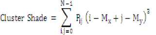
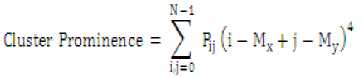
where М^^Щ,- and My:^

The above statistical features analyze the spatial distribution of gray values, by comparing local features at each point in the image. The reason behind this is the fact that the spatial distribution of gray values is one of the defining qualities of texture. In order to improve the classification gain the combination of feature vectors F 1 and F 2 is used as feature vector F 3 in the present paper.

In the classification phase, an unknown texture is used and its features are extracted and compared with the corresponding feature values stored in feature library using a Euclidean distance vector formula given in Eqn.(16).

Table 1.

S.No	Images	Classification gain(%)
		F 1	F 2	F 3
1	Bark.0006	92.9	96.4	95.2
2	Brick.0000	73.8	96.4	96.4
3	Brick.0004	77.4	81.0	78.6
4	Clouds.0001	91.7	96.4	94.1
5	Fabric.0013	100.0	100.0	100.0
6	Fabric.0017	88.1	61.9	96.4
7	Flowers.0006	96.4	96.4	100.0
8	Food.0000	100.0	92.9	100.0
9	Food.0001	91.7	86.9	98.8
10	Grass.0001	100.0	61.9	92.9
11	Leaves.0012	96.4	95.2	100.0
12	Metal.0002	89.3	91.7	98.8
13	Metal.0004	97.6	97.6	100.0
14	Misc.0001	97.6	83.3	100.0
15	Misc.0002	100.0	77.4	100.0
16	Sand.0000	95.2	57.1	96.4
17	Sand.0002	94.1	66.7	98.8
18	Tile.0008	96.4	84.5	98.8
19	Water.0005	100.0	96.4	100.0
20	Wood.0002	100.0	90.5	100.0
Average		93.93	85.54	97.26
Number of image regions correctly classified		1578	1437	1633

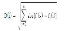
where n is the total number of features used, i = 1 to Q

Using the feature vector F 1 , F2, F 3 the success rate achieved is 93.93%, 85.54, 97.26% respectively. The classification result of Dataset-2 and Dataset-3 are given in the Table 2 and 3 respectively. The classification results exhibits the same tendency as Dataset-1

Table 2: Results of texture classification using Dataset-2 of first and second order features (1680 image regions)

S.No	Images	Classification gain(%)
		F 1	F 2	F 3
1	D 1	95.83	91.67	100.0
2	D 2	91.67	91.67	97.6
3	D 3	95.83	91.67	78.6
4	D 4	94.1	66.7	97.6
5	D 5	96.4	84.5	100.0
6	D 6	94.8	96.4	100.0
7	D 7	90.7	93.4	100.0
8	D 8	95.83	91.67	97.6
9	D 9	91.7	86.9	97.6
10	D 10	100.0	61.9	81.0
11	D 11	96.4	95.2	100.0
12	D 12	89.3	91.7	98.8
13	D 13	97.6	97.6	100.0
14	D 15	97.6	83.3	98.8
15	D 16	100.0	77.4	98.8
16	D 17	95.83	87.5	100.0
17	D 18	87.5	87.5	97.8
18	D 19	87.5	91.67	97.8
19	D 20	91.67	91.67	96.5
20	D21	81.9	92.9	100.0
Average		93.61	87.65	96.93
Number of image regions correctly classified		1564	1472	1628

Table 3: Results of texture classification using Dataset-3 of first and second order features (with 1680 image regions)

S.No	Images	Classification gain(%)
		F 1	F 2	F 3
1	G 1	92.9	86.5	98.7
2	G 2	94.1	94.7	97.6
3	G 3	96.4	84.5	100.0
4	G 4	89.5	92.9	97.6
5	G 5	95.2	57.1	100.0
6	G 6	94.1	66.7	97.6
7	G 7	96.4	84.5	100.0
8	G 8	100.0	92.9	97.6
9	G 9	91.7	86.9	97.6
10	G 10	95.8	91.7	100.0
11	G 11	91.7	91.7	97.6
12	G 12	95.8	91.7	78.6
13	G 13	97.6	97.6	100.0
14	G 14	98.5	83.3	98.8
15	G 15	100.0	77.4	98.8
16	G 16	95.2	57.1	100.0
17	G 17	94.1	66.7	97.6
18	G 18	96.4	84.5	100.0
19	G 19	100.0	96.4	100.0
20	G 20	100.0	90.5	100.0
Average		95.8	83.8	97.9
Number of image regions correctly classified		1608	1407	1645

A. Comparision of the proposed FLRTUM with other Methods

Table 1,  2 and 3 shows the mean percentage classification rate for each group of textures by using the proposed AFLRTU. Other existing methods of CDTS [21] and modified CDTS [22] method applied on VisTex, Brodatz and Granite texture database images are represented in Table 4 respectively. From Table 4, it is clearly evident that, the proposed AFLRTU exhibits a high classification rate than the existing methods. The graphical analysis of the percentage mean classification rate for the proposed AFLRTU and other existing methods of three databases are shown in Fig.6.

Table 4: Comparison of the proposed AFLRTU method with the existing methods.

Database	CDTM	Modified CDTM	Proposed AFLRTU Method
VisTex	84.92	92.6	96.79
Brodatz	87.56	92.26	96.93
Granite	75.71	90.32	97.90

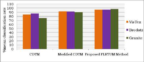
Fig.6: Comparison of proposed AFLRTU and existing methods.

• IV.    Conclusions

  The present paper derived a new AFLRTU to overcome the disadvantages of FTU, LRTM and CDTM. The AFLRTU approach considers two sets of four connected texture elements on a 3×3 grid for evaluating the TU instead of non-connected or corner texture elements as in the case of Cross Diagonal Texture Matrix (CDTM) or Modified CDTM. The AFLRTU reduced the size of TU from 2020 to 79 as in the case FTU, thus it reduced the overall complexity. The AFLRTU achieved rotational invariance by considering the average of all four combinations of TU, which is missing in LRTM. This feature extraction process is quite efficient with less complexity. When compared with other approaches, the proposed scheme is more effective and exhibiting increased classification ability by using smaller feature vectors. The experimental results prove the efficacy of the proposed method when compared to several other methods.

Acknowledgment

The authors would like to express their gratitude to Sri K.V.V. Satya Narayana Raju, Chairman, and K. Sashi Kiran Varma, Managing Director, Chaitanya group of Institutions for providing necessary infrastructure. Authors would like to thank anonymous reviewers for their valuable comments and Dr. G.V.S. Ananta Lakshmi for her invaluable suggestions which led to improvise the presentation quality of this paper