A new Decision Based Median Filter using Cloud Model for the removal of high density Salt and Pepper noise in digital color images

Image Denoising is the process of removing the noise from the digital images using some prior knowledge about the noise while retaining as much as possible important image features. Basically, there are two approaches to image denoising based on the domain in which the denoising taken place. These approaches are named as spatial domain and transform domain filtering approaches. Spatial Filtering approaches remove the noise by manipulating the image in the spatial domain itself, whereas Transform Filtering approaches manipulate the image in transform domain.

Spatial filtering of images is an important aspect of image processing as it provides means for removing noise and sharpening blurred images. There are many types of spatial filters which can be classified into linear and non-linear filters. The simplest linear spatial filter is mean filter [1], which works by passing a mask over the image calculating the mean intensity and setting the central pixel to this value. They tend to remove the fine details in the image and fail to remove high level noise effectively. Among spatial filters, the famous non-linear filter is standard median filter (SMF) [2].

SMF is similar to mean filter but it replaces the centre pixel of the window by the median value of the window. The main drawback of SMF is that it exhibits blurring by removing the lines and corners in the image while suppressing the noise. To overcome this drawback, several variations of SMF have been proposed.

The weighted median filter (WMF) is one of the extensions to median filter which assigns more weights to some pixels in the window [3, 4]. This WMF provides some degree of control to the smoothing behaviour through the weights assigned. These weights introduce additional complexity in the design and implementation of WMF. Another variation of SMF is the Centre Weighted Median Filter (CWMF), which gives more weights to the central value of the window only, thereby reduces the complexity in the design [5]. The CWMF filter performs well for low noise level and fails when the noise level is high. To overcome this, Adaptive Median Filters (AMF) with variable window size was introduced [6].

AMF is robust in removing the impulse noise while preserving the image details even though the probability of occurrence of impulse noise is high. The filters discussed above unconditionally replace each pixel with median value of the window without checking whether the pixel is “bad” or not. As a result, since the uncorrupted pixels are altered, they damage many image details in the high noise levels. To avoid the damage of uncorrupted pixels, the use of switching filters were introduced. These filters employ an impulse detector to determine the presence of pixels corrupted by impulses in the image. Only these noisy pixels will be filtered by these switching filters.

The Progressive Switching Median Filter (PSMF) is one of the switching filters in which both impulse detector and noise filter are applied progressively in iterative manner to obtain the best results [7]. These progressive iteration increases the time complexity of the filter. Again, in switching filters, the noisy pixels are replaced by median value without taking the local features into account. At higher noise densities, the median value of the window may also be a noisy pixel.

To overcome this problem, decision based median filter (DBMF) was proposed to replace the corrupted pixels by either the median pixel or left neighborhood pixel [8]. Although this filter shows promising results, smooth transition between the pixels is lost leading to degradation in the visual quality of the image. To provide smooth transition between the pixels with edge preservation and better visual quality, a modified decision based median filter (MDBMF) was proposed in which noisy pixel is replaced by the median pixel or the mean of the neighborhood processed pixels [9]. The noisy pixel replacement by the mean of the neighborhood processed pixels will lead to blurring of the edges and fine details in the image. To preserve the edges and fine details, this paper proposes and implements a new decision based median filter using cloud model to restore the highly corrupted digital color images. The proposed filter is tested on different images and shows better performance than standard median filter, adaptive median filter, decision based median filter and modified decision based median filter in terms of root mean square error, peak signal to noise ratio and image quality index.

The remaining portion of the paper is organized as follows. The second section of this paper discusses about cloud model and its parameters. The proposed new decision based median filter is described in third section. The evaluation criteria and the results of the proposed filter are presented in fourth and fifth section of this paper. The last section concludes the paper.

• II.    CLOUD MODEL

To remove the impulse noise in the digital images, it is necessary to grasp the impulse noise characteristics. Uncertainties are inherent features of impulse noise [10]. So, understanding the uncertainties and apply them in a better way can improve the performance of impulse noise removing filter. Uncertainties in impulse noise exist through the randomness and the fuzziness. The fact that the pixels are randomly corrupted and randomly set to the maximum or minimum extreme value shows the randomness whereas not all of the extreme value pixels are the noisy pixels shows the fuzziness associated with impulse noise. The relationship between the randomness and fuzziness was established by Cloud Model (CM) [11]. CM is a model of the uncertainty transformation between quantitative representation and qualitative concept based on normal distribution and bell shaped membership function. CM has been successfully applied to data mining [12, 14], image classification [13], image segmentation [15, 16] and optimization [17].

Let U is a quantity domain expressed with accurate numbers and C is a quality concept in U. If the quantity value, x ϵ U and x is a random realization of the quality concept C, then μ ( x ) is the membership degree of x which lies between [0,1]. It is the random number which has the steady tendency,

µ : U → [0,1], ∀ x ∈ U , x → µ ( x )                   (1)

The distribution of x is called cloud and each x is called a cloud drop. The cloud can be characterized by three parameters, i.e., the expected value Ex, entropy En, and hyperentropy He [10-17]. Ex is the expectation of the cloud drops’ distribution. It points out which drops can best represent the concept and reflects the distinguished feature of the concept. En is the uncertainty measurement of the qualitative concept, which is determined by both the randomness and the fuzziness of the concept. It represents the value region in which the drop is acceptable by the concept, while reflecting the correlation of the randomness and the fuzziness of the concept. He is the uncertainty measurement of En. Given these three characteristics, a set of cloud drops can be generated with certainty degree by the normal cloud generator CG. Each pixel in the image is the cloud drop and composes the cloud. These cloud drops are given input to the backward cloud generator CG-1. The outputs of CG-1 are three parameters of cloud Ex, En and He. This is shown in Figure 1.

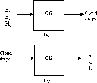
Figure 1. (a). Forward Cloud Generator (b). Backward Cloud Generator

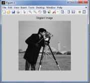
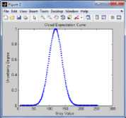
When the drops are approaching the expected value E x , the certainty degrees and the contribution degrees of the drops are increasing. Therefore, the drops in the cloud contribute to the concept with the different contribution degrees [20]. The drops located within [E_x-3E_n, E_x+3E_n] take up to 99.99% of the whole quantity and contribute 99.74% to the concept. Thus, the drops are located out of domain [E_x-3E_n, E_x+3E_n], and their contributions to the concept can be neglected. This is “3En rule.” According to the normal cloud generator (CG), the certainty degree of each drop is a probability distribution rather than a fixed value. It means that the certainty degree of each drop is a random value in a dynamic range. If H e of the cloud is 0, then the certainty degree of each drop will change to be a fixed value. The fixed value is the expectation value of the certainty degree. In fact, the value is also the unbiased estimation for the average value of the certainty degrees in the range. A curve called cloud expectation curve (CEC) can be constructed by plotting all the drops in X-axis and their expectations of certainty degrees in Y-axis. The CEC of cameraman image is shown in the Figure2.

(a)

(b)

Figure 2. (a).Cameraman Image (b).CEC

filtering window    W_t ² N + 1  of size 2 N + 1.

W2N+1 = {xi+s,j+1} where s,t e (-N,...0,..N) .

Step 1: Set the window size by initializing N =1. Then,

E x of each uncorrupted pixels in W^²N ^{+ 1}

is calculated

using the formulae,

Ex

• III.    PROPOSED NEW DECISION BASED NEDIAN FILTER

The proposed new decision based median filter (PNDBMF) is a two stage filter, where the first stage is the noisy pixel detector and the second stage is the noisy pixels replacement filter. In the first stage, each pixel is tested to find whether the pixel is noisy or noise-free. When a pixel is classified as noise-free, it will be retained and the filtering action is avoided without altering any fine details and textures that are contained in the original image. When a noisy pixel is detected in the first stage, then the median value of the window is also tested. If the median value of the window is not noisy, then the noisy pixel is replaced by median value of the window. Otherwise, the noisy pixel is replaced by the value ‘0’ and passed to the next stage for filtering.

• A.    Noisy Pixel Detector

Similar to other impulse detection algorithm, this Noisy Pixel Detector (NPD) uses prior information about the impulsive noise with the following assumptions.

• •    Only the proportions of image pixels are corrupted while other pixels are noise free.

• •    Noisy pixels take a very large value as positive impulse or a very small value as negative impulse.

Normally, the impulse noise is modeled as salt and pepper noise. The salt noise takes the pixel value of 255 and pepper noise takes the pixel value of 0. These two pixel values are used to identify the noisy pixels in the image. The NPD checks the value of every pixel in the image. If the pixel value is ‘0’ or ‘255’, the pixel is classified as noisy pixel. Otherwise the pixel is classified as noise free pixel. When a pixel is classified as noise free, it will be retained without altering any fine details and textures in the original image. When a noisy pixel is detected in the first stage, then the median value of the window is also tested. If the median value of the window is not noisy, then the noisy pixel is replaced by median value of the window. Otherwise, the noisy pixel is replaced by the value ‘0’ and passed to the next stage for filtering.

• B.    Noisy Pixel Replacement Filter

The Noisy Pixel Replacement Filter (NPRF) replaces the noise pixel with the value ‘0’ by the weighted fuzzy mean value of the remaining pixels in the square

1 n

x

z

i + s,j + t e

W2N + 1 i,j

^xi + s,j + 1

Step 2: Calculate E n using the following formulae,

E n = ^{x          z         x}i + s,j + 1  ^Ex|

² n     . _w2N + 1

^xi + s,j + t e ^Wi,j

Step 3: Calculate weights for xi + _s,j + t

^wi + s,j + 1 = ^{exp( (x}i + s,j + t  Ex) ^/2En)           ⁽⁴⁾

Step 4: Calculate the weighted mean

Yi,j =        z xi+s,j+teW2N+1

wi+s,j+txi+s,j+t /

/ wi+s,j+1

Step 5: Replace the noisy pixel value by weighted mean .

mean Y_{i , j} .

IV. EVALUATION CRITERIA

The following evaluation measures are used in this paper. The Root Mean Square Error (RMSE) between the reference image R and fused image F is given by,

RMSE=

NN

Z Z [R(i,j) — F(i,j)]2

i = 1j = 1

N2

The Peak Signal to Noise Ratio (PSNR) between the reference image R and fused image F is given by,

PSNR= 10log 10 (255) ² /(RMSE) ² (db)               (7)

Quality index of the reference image (R) and fused image (F) is given by [18],

QI=        ^4σ ab ^ab

(a ² + b ² )(^a ² + ^b2)

The maximum value Q=1 is achieved when two images are identical, where a & b are mean of images, σ _ab be covariance of R & F, σ _a , σ _b be the variance of image R,F.

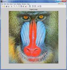
a. Mandrill

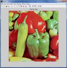
b. Pepper

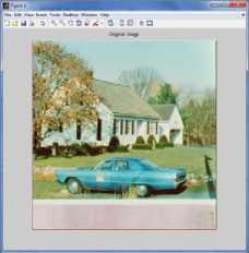
c. House

Figure 3. Original Images

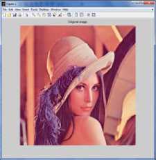
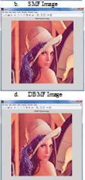
d. Lena

MDBMT Ьаи        f. ЮТБМГ Ьме

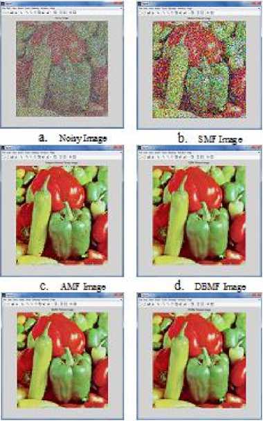
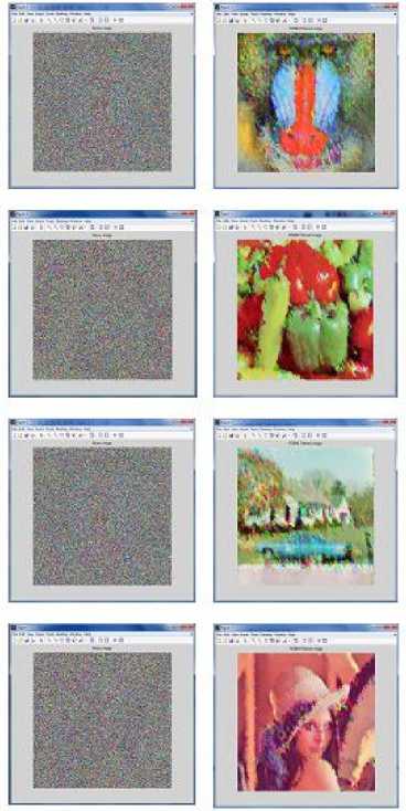
Figure 5. Results of various filtered Images for pepper image of noise density 75%

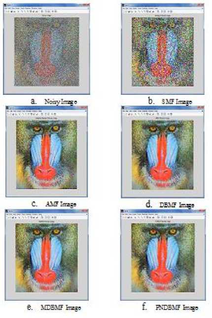
Figure 4. Results of various filtered Images for mandrill image of noise density 75%

е. ХЮВМГЬж        f B-TElJb=»

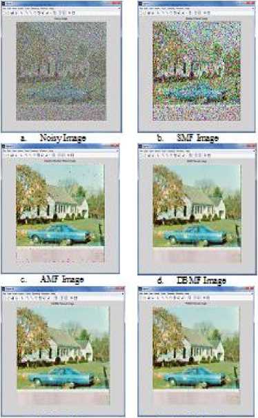
Figure 6. Results of various filtered Images for house image of noise density 75%

TABLE I. PERFORMANCE COMPARISON TABLE FOR MANDRILL IMAGE AT DIFFERENT NOISE DENSITIES

Noise	0.75	0.8	0.85	0.9	0.95
RMSE
Noisy	120.72	124.651	128.502	132.129	135.699
SMF	94.1488	103.638	112.849	121.871	130.55
AMF	31.5887	38.2727	49.7289	68.0547	95.6429
DBMF	29.1042	31.405	34.3988	38.3776	44.8895
MDBMF	28.803	30.9906	33.843	37.4185	43.4878
PNDBMF	28.7143	30.7673	33.3327	36.1653	40.1523
PSNR
Noisy	6.4968	6.2186	5.954	5.7123	5.4807
SMF	8.6557	7.8224	7.0818	6.4141	5.8165
AMF	18.1559	16.4803	14.1999	11.4772	8.5193
DBMF	18.8755	18.214	17.4231	16.4754	15.1166
MDBMF	18.9655	18.3288	17.5666	16.6941	15.3894
PNDBMF	18.9926	18.3907	17.6978	16.9899	16.0863
QI
Noisy	0.0941	0.0721	0.0512	0.0341	0.0172
SMF	0.2526	0.1866	0.1293	0.0818	0.041
AMF	0.8313	0.7658	0.6428	0.4572	0.2287
DBMF	0.8511	0.8267	0.7928	0.7453	0.6538
MDBMF	0.8536	0.8304	0.7979	0.7545	0.6692
PNDBMF	0.8549	0.8333	0.8046	0.771	0.7169

TABLE II. PERFORMANCE COMPARISON TABLE FOR PEPPER IMAGE AT DIFFERENT NOISE DENSITIES

Noise	0.75	0.8	0.85	0.9	0.95
RMSE
Noisy	122.586	129.247	133.346	137.073	140.795
SMF	94.0307	105.908	116.306	125.656	135.137
AMF	23.9472	29.2673	44.6285	66.0374	97.3284
DBMF	22.2268	20.4416	24.274	30.3079	40.3
MDBMF	22.0389	20.0305	23.7984	29.4482	39.0779
PNDBMF	21.76	19.4516	22.2675	26.7154	33.6652
PSNR
Noisy	6.3622	5.9081	5.637	5.3978	5.1648
SMF	8.6655	7.637	6.8241	6.1529	5.5205
AMF	20.5486	18.825	15.1546	11.7506	8.3746
DBMF	21.2015	22.0745	20.593	18.7214	16.2463
MDBMF	21.2755	22.2516	20.7576	18.9477	16.4749
PNDBMF	21.388	22.5026	21.3278	19.7599	17.7644
QI
Noisy	0.089	0.0702	0.0491	0.0322	0.017
SMF	0.2642	0.1978	0.1329	0.0856	0.0436
AMF	0.8979	0.8536	0.7027	0.4933	0.2464
DBMF	0.909	0.9266	0.8966	0.8417	0.7177
MDBMF	0.9104	0.9295	0.8999	0.8484	0.7279
PNDBMF	0.9129	0.9334	0.9123	0.874	0.7988

TABLE III. PERFORMANCE COMPARISON TABLE FOR HOUSE IMAGE AT DIFFERENT NOISE DENSITIES

Noise	0.75	0.8	0.85	0.9	0.95
RMSE
Noisy	122.599	126.645	130.468	134.295	137.961
SMF	94.0083	104.105	113.763	123.371	132.602
AMF	24.189	31.6178	45.1788	65.492	95.1604
DBMF	22.2148	25.0528	28.5946	34.2598	43.7103
MDBMF	22.0201	24.7395	28.2373	34.0619	43.281
PNDBMF	21.7035	24.1939	26.9062	31.5053	37.8527
PSNR
Noisy	6.3614	6.0793	5.8211	5.5699	5.336
SMF	8.6676	7.7816	7.0111	6.3068	5.6802
AMF	20.4606	18.1338	15.0343	11.8073	8.5629
DBMF	21.2054	20.1557	19.0128	17.4385	15.3236
MDBMF	21.2821	20.2657	19.1228	17.4891	15.4117
PNDBMF	21.4085	20.4604	19.5399	18.1676	16.5722
QI
Noisy	0.0891	0.0685	0.0501	0.0319	0.0158
SMF	0.2646	0.1967	0.1395	0.0861	0.0431
AMF	0.8957	0.8308	0.6953	0.4885	0.2449
DBMF	0.9089	0.8848	0.8506	0.7854	0.656
MDBMF	0.9103	0.8873	0.8534	0.7861	0.6557
PNDBMF	0.913	0.8928	0.8676	0.8185	0.7438

TABLE IV. PERFORMANCE COMPARISON TABLE FOR HOUSE IMAGE AT DIFFERENT NOISE DENSITIES

Noise	0.75	0.8	0.85	0.9	0.95
RMSE
Noisy	121.47	125.599	129.46	133.198	136.924
SMF	92.7514	103.163	112.9	122.374	131.823
AMF	17.7353	26.9811	41.8173	63.2114	94.4781
DBMF	14.0953	16.7304	19.5351	24.0599	32.7897
MDBMF	13.8682	16.3605	19.1632	23.4925	32.6373
PNDBMF	13.5161	15.864	18.0859	21.1386	26.3262
PSNR
Noisy	6.4472	6.1569	5.8937	5.6465	5.4075
SMF	8.7911	7.8668	7.0822	6.3826	5.7382
AMF	23.1732	19.5159	15.7075	12.1209	8.6329
DBMF	25.1803	23.7122	22.3739	20.5713	17.89
MDBMF	25.3207	23.9051	22.5437	20.7648	17.929
PNDBMF	25.5403	24.1699	23.0471	21.6808	19.8115
QI
Noisy	0.0672	0.0514	0.0364	0.0234	0.0114
SMF	0.2101	0.1521	0.1035	0.0632	0.0288
AMF	0.921	0.8297	0.6582	0.4286	0.198
DBMF	0.9483	0.9285	0.9025	0.8534	0.7302
MDBMF	0.9499	0.9314	0.9062	0.8583	0.7322
PNDBMF	0.9523	0.9352	0.9164	0.8847	0.8227

о MDBMF brass

£ PNTBMF brass

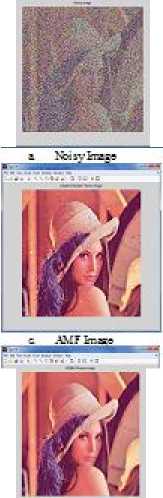
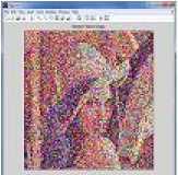
Figure 7. Results of various filtered Images for lena image of noise density 75%

• V.    RESULTS

• VI.    CONCLUSIONS

In this paper, a new decision based median filter for removal of high density salt and pepper has been proposed and implemented. This filter represents the uncertainties of the salt and pepper noise perfectly by using cloud model, which is essential in removing the noise. In addition, the above filter identifies the noise pixel directly, without any need to sort the pixel gray values, which immensely increases the computational efficiency in noise detection. Even if the noise density is close to 0.95, the texture, details and edges of the images are preserved with good visual effect as shown in figure 7. In total, the proposed filter is a moderately simple denoising filter with good detail preservation.

ACKNOWLEDGMENT

The author thanks anonymous referees for their comments and suggestions.