A New Locally Adaptive Patch Variation Based CT Image Denoising

Computed Tomography (CT) is an important tool to detect the internal problems in human body such as depiction of lesions in human organs, skull fracture, brain hemorrhage and many more. CT scan images provide extraordinary sensitive medical relevant information which may helpful to diagnose the problems. However, high radiation dose, low contrast, noise and artifacts are some major drawbacks in computed tomography. Still, it is widely used because of low cost, easy availability, short execution time and excellent sharp images. The impact of radiation dose is directly related to CT image quality. High radiation dose may improve the image quality but it may harm to patients. Low radiation dose may degrade the image quality in terms of noise. Due to noisy CT images, the experts may not comfortable to diagnose the problems.

Various techniques have been investigated to control the noise in CT scan imaging. Projection based techniques such as projection space denoising with bilateral filtering and CT noise modeling for dose reduction in CT imaging [1] work on raw data or sinogram, where noise filtering is performed on raw data or sinogram and the denoised image is reconstructed. Many iterative reconstruction approaches for noise suppression in CT have also been proposed such as ordered subset based reconstruction for X-ray CT scan [2] optimizes the statistical functions and improve low dose CT images. Most of other techniques e.g., bilateral filtering [1, 3], total variation denoising [4, 5], nonlocal means (NLM) denoising [6, 7] and k-SVD [8] take the advantages of statistical properties of objects in image space and preserve clinical structures such as sharp edges, similarities between neighboring pixels, etc. In transformdomain denoising techniques, the input data is decomposed into its scale-space representation [9]. Linear filters such as Wiener filter [10] in the wavelet domain give optimal results when the signal distortion is estimated as Gaussian approximation and the accuracy is measured by calculating Mean Square Error (MSE). Various thresholding techniques for noise reduction have also been introduced with wavelet transform such as efficient image denoising method based on a new adaptive wavelet packet thresholding function [11, 12], ideal spatial adaptation via wavelet shrinkage [13, 14] etc. Thresholding is one of the important tools for denoising. VISUShrink [13,  15] is a non-adaptive universal threshold, which depends only on number of samples and known to find smoothed images because its threshold choice can be large due to its dependence on the number of pixels in the images. SUREShrink [13, 16] uses a hybrid of the universal and the SURE [Steins Unbiased Risk Estimator] thresholds, and performs better than VISUShrink. BayesShrink [17-19] minimizes the Bayes risk estimator function assuming generalized Gaussian approximation and thus finds adaptive threshold value. Chang et al. [20] proposed the use of adaptive wavelet thresholding for image denoising, by modeling the wavelet coefficients as a generalized Gaussian random variable, whose parameters are estimated locally (i.e., within a given neighborhood). In image space, CT images can be denoised directly without access to raw data. CT image denoising is a challenging task because of finding correct noise variation, relationship between coefficients and achieving an optimal trade-off between denoising and blurring or artifacts [21-23]. To surmount these challenges, we propose a maximum edge preserving and noise reduction method. Experimentally, it is observed that each wavelet coefficients are affected with different patch size. With different patch size, the estimated threshold value may not be the same and may affect images in terms of local features and noise. With this consideration, we propose a scheme for CT image denoising based on the variation in multiple thresholded values which are obtained by different patch sizes.

The paper is organized as follows. Section 2 gives a brief overview of wavelet based shrinkage. In section 3, the proposed method is presented in details. Experimental results, including discussions and comparison with other denoising methods, are given in section 4. Finally, conclusions are summarized in section 5.

• II.    Image Denoising by Wavelet Shrinkage

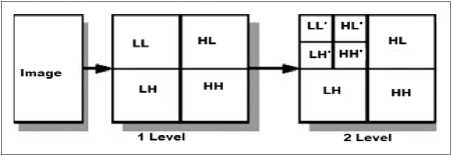
Wavelet transform is a powerful tool for signal and image processing tasks because of multi-resolution analysis, sub-banding and localized in both, frequency and time domain. Two dimensional DWT transforms the signals into low frequency (LL) and high frequency components (LH; HL; HH), as shown in Fig. 1.

With the assumption, the CT images are corrupted by Gaussian noise with zero mean and different variances, the noisy CT image can be expressed as:

X (m, n ) = Y (m, n) + rm m, n) (1)

Where, n(m , n ) is a noise coefficient, Y ( m, n ) and X ( m , n ) are noiseless and noisy images respectively.

Before applying wavelet thresholding, two important tasks must be performed which are responsible for the results and computational complexity. First, a wavelet basis is chosen for determining its decomposing layers such as haar, db2, etc. Second, decomposition level is chosen for thresholding on all subbands for all levels. Wavelet based noise shrinkage can be expressed with the following major steps:

Step 1: Perform discrete wavelet transform (DWT) on input noisy CT image to obtain approximation and detail parts.

Step 2: Perform the denoising using following steps:

• i.    Estimate noise variance

• ii.    Apply thresholding on detail parts

Step 3: Apply inverse discrete wavelet transform (Inverse DWT) to obtain final denoised image.

A. Threshold Selection

For CT images, selection of a threshold value is not an easy task. By selecting small threshold value, the resultant image may be noisy. For large threshold value, the resultant image may blur on the edges. The selection of optimal threshold value is necessary and important task for preserving clinical details and suppression of noise.

The threshold X can be selected as:

X =

° -

I O J

Where the noise variance can be estimated using robust median estimation method (Abramovitch et al. 1998) as follows:

°-

median (| X(m, n) |)0.6745

Where, X ( m , n ) ϵ HH , L represents respective level in wavelet decomposition. The standard deviation of noise less image ( c r_r) can be estimated as:

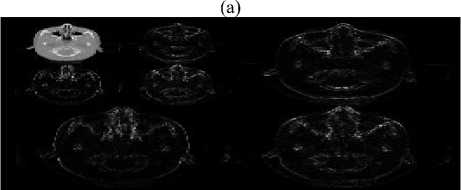
(b)

Fig.1. (a) First and Second Level 2-D Wavelet Decomposition (b) 2D-DWT Decomposition on CT image up-to two levels.

o Y = max( o 2 - o ², 0)

Where, _o 2 =      X ² and b represent patch size

X                  i, b i=1

of an input image.

B. Threshoding process

After selecting a threshold value, the process of

thresholding is applied by selecting an appropriate algorithm. Hard thresholding and soft thresholding methods are very popular for thresholding. In hard thresholding, each coefficient value is compared with threshold value and values less than threshold are replaced by zero. In Soft thresholding, replacement process is same as in hard thresholding, additionally rest of coefficients are modified by subtracting threshold values. In comparison of both, Soft thresholding gives better performance for visual appearance of images. The soft thresholding can be expressed as:

л I 0

Y := 1

I sign ( X )( X - 2 )

ifX <  ifX >

• III.    Proposed Methodology

The perfect optimization for estimating a threshold value is an almost impossible task for image denoising. Estimated threshold value may be varying according to different patch sizes. With the consideration that the small variation of neighborhood size will not much affect the threshold estimated value, a new locally adaptive different patch size based thresholding scheme is proposed, where some limited patch sizes are selected. The patch sizes can be extracted as: If X ( m , n ) is the size of image, then for high frequency subband’s first patch size will be ( m /2, n /2) . Similarly, k — 1 numbers of subband are generated by dividing previous patch size by 2.

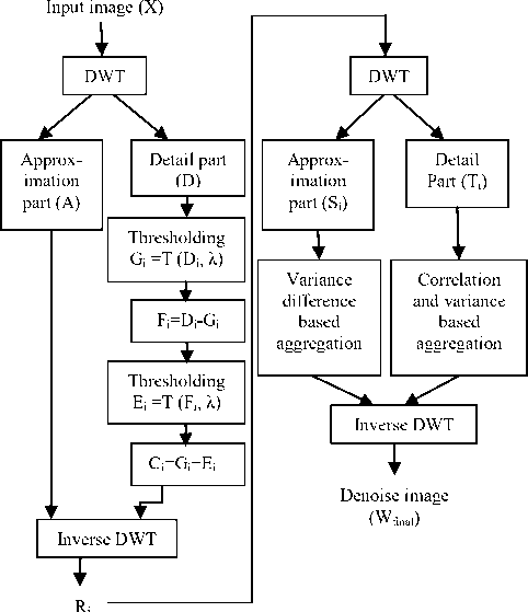
Fig.2. Flow Chart of Proposed Scheme

With the assumption, that the CT image is corrupted by

Gaussian noise, the proposed method as shown in fig. 2 can be summarized as:

• 1)    Select the maximum size of input noisy CT image X ( m , n ) where m = 2 ^k and n = 2 ^k .

• 2)    Apply DWT on input image to obtain low frequency ( A ) and high frequency ( D ) subbands.

• 3)    High frequency subbands ( D ) are patching wise threshold (for i = 1 to k — 1 ) using equation (5) according to respective patch size.

G t = T ( D i , 2 )                  (6)

Where, λ is an estimated noise level calculated using equation (3).

• 4)    Apply method noise using input high frequency ( D ) subband and thresholded high frequency subband ( G_i ) as:

• i)    Subtract G from D and get F as,

F. = D — Gi

• ii)    Apply patch wise thresholding on F .

Ei = T (Fi, 2)

• iii)  Add G and E and get C ,

Ci = Gi + Ei(9)

• 5)    Apply inverse DWT, using low frequency ( A ) and thresholded high frequency ( C ) subbands. The output ( R. ) comes in the form of k — 1 denoised images.

• 6)    To obtain final denoised image, perform the following steps:

• i)    Separately apply DWT on R images to obtain their approximation ( S ) and detail parts ( T ).

• ii)    Estimate the variance at each pixel of approximation part at level 2 of all denoise images ( R ) in block of size 3 × 3.

• iii)    Variance ( Var ) difference on approximation part of denoised images ( R ), as below:

1     k —2

^T = k ^2 ^:^ =? “ j              ⁽¹⁰⁾

where,

The value of T is normalized in the range [0 1] and used as a weight factor for the next process.

iv) Variance difference based aggregation process is based on weight factors T and perform on approximation part as per the following relationship:

Bf / = h + Q final

where,

k - 1

k - 1

k - 1

z

k - , g=T+1

—

T

^{( k —} g )

( S g )

v) Variance based aggregation (Jain et al. 2015) using correlation (Corr) is performed on detail parts using following relationship:

ГT1 b,        If Corr(Ti, Ti+1)>Th final |z ebTb,  Otherwise

I i = 1

images are obtained. To get final denoised image, separately DWT is performed on all denoised images. In approximation part of all denoised images, a weight value T is estimated using variance difference between different denoised images. This weight value is incorporated into denoised images and aggregation relationship has been performed as shown in Step 6(iv). In detail part, patch wise correlation coefficient values are obtained between all denoised images. Correlation value lies in the interval [-1; 1], where 1 means perfect correlation, 0 no correlation, and -1 perfect anticorrelation. To find correlated and uncorrelated values, correlation values are normalized in the range of [0; 1]. The correlation values closer to 1 indicate that the similarity structure is present between the images. The lower values (near to 0) indicate that the corresponding value includes only noise and, therefore, can be suppressed. If correlation value is greater with a defined threshold ( T ) value then keep the largest patch size denoised coefficient value of subband, otherwise, perform variance based weighted average between all denoised coefficients of subband as given in Step 6(v). Thus, final denoised CT image can be obtained using inverse wavelet transform.

IV. Experimental Results

where, в =

k - 1

Z Var ЛТ )

i = 1

T represents detail part of all denoised images ( R ) with block size b . T represents a defined threshold value to differentiate between correlated and uncorrelated coefficients. The function Var ¹ (.) can be estimated as inverse variance.

• 7)    Apply inverse DWT using B_final and C_final to obtain final denoised image ( W ).

In proposed scheme, noisy CT image is denoised in wavelet domain where noise on high frequency coefficients of each subband in L level has been suppressed using Bayes shrink and method noise thresholding with different patch sizes. In method noise, the thresholded patch is subtracted with original patch. The outcome of subtraction is again thresholded and added into the thresholded original patch. This method noise thresholding process is used to observe, how much local features of clinical details are missing at the time of thresholding and can be recovered as shown in Step 4. With different patch size, separate multiple denoised

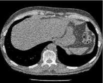
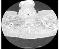
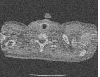
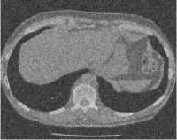
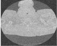
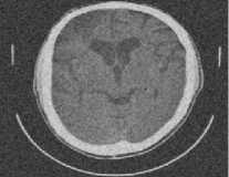
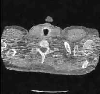
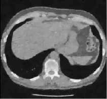
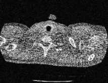
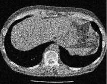
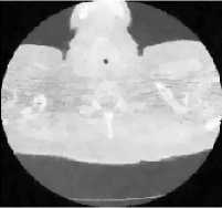
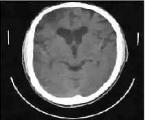
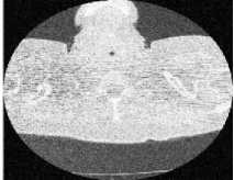
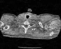
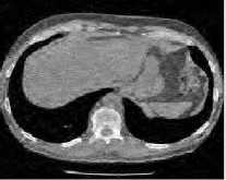
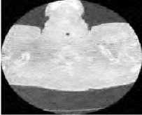
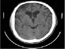
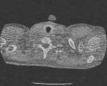
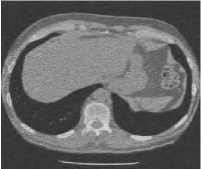
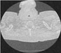
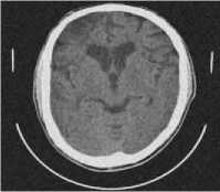
The experimental evaluation is performed on low quality CT images with size512x512. The CT scanned test images shown in fig.3(a-c) is obtained from public access database cgi), and CT scanned test image shown in fig. 3(d) is obtained from a Diagnosis Center. The proposed image denoising method is applied on all test images corrupted by additive Gaussian white noise at six different noise level (σ): 10, 15, 20, 25, 30, and 35. Fig. 3(a), 3(b), 3(c) and 3(d) are considered as CT images 1, 2, 3 and 4, respectively. Fig. 4(a-d) are showing noisy test image data set with σ = 25.

(a) CT 1 image

(b) CT 2 image

(c) CT 3 image

Fig.3. Input Test CT Image Dataset

(d) CT 4 image

(a) CT 1 image

(b) CT 2 image

Image quality index (IQI) is another important factor to analyse the performance of image denoising in terms of correlation, luminance distortion and contrast distortion. For input image (X) and denoised image (W), the IQI can be defined as:

(c) CT 3 image

(d) CT 4 image

Fig.4. Noisy CT Image Dataset (σ=25)

where,

IQI =

4^xwXW

(^X + ф2)[( x )2 + (W )2]

N

x=- УЛ Ni

—

i = 1

—        N,

W=N SW, "X

—

N

• A.    Evaluation of different patch size

k — 1 numbers of patch sizes are used to denoise the images using proposed methodology. The outcome of thresholding may be differ with differ local patch sizes. As k — 1 numbers of patch size are used separately for thresholding, k — 1 numbers of thresholded subband are obtained respectively. To verify the effect of different patch sizes for thresholding, an average correlation value is obtained between k — 1 thresholded subband for all test images. Table 1 shows the average values of the correlations using a 7x7 window for all CT image dataset.

Table 1. Average Values of the Correlations between K-1 Denoised Images using Different Patch Size

Level (L)	L=1	L=2	L=3	L=4
CT 1 image	0.9501	0.9385	0.8976	0.8793
CT 2 image	0.9729	0.9462	0.8991	0.8592
CT 3 image	0.9201	0.8976	0.8715	0.8358
CT 4 image	0.8973	0.8695	0.8413	0.8187

• B.    Performance evaluation

Peak Signal-to-noise Ratio (PSNR) is an important factor to evaluate denoising performance. The high PSNR value represents more similarity between the denoising and original image than lower PSNR value. The objective quality of the denoised image is measured by PSNR as:

PSNR = 10 log10---- dB mse

Where mse is the mean square error between the original and the denoised image:

mn

mse = SS [X(-, j) — W(-, j)]2   (14)

mn i = 1 j = 1

and

N       —        —

N ^{— 1} - = 1

The quality of image index range lies between 1 and -1. The highest value 1 represents an identical value of input image pixel and denoised image pixel. The lowest value -1 shows that the pixels values are uncorrelated.

• C.    Experimental evaluation

To evaluate the results of proposed scheme, the parameters are kept fixed throughout the comparisons as in other methods. The result evaluation is performed on the CT images with the size of 512x512, can be expressed as 2 ⁹ x2 ⁹ . As per proposed scheme, we can evaluate the total number of patch sizes are k-1 i.e 8 and patch size can be expressed as: 256x256, 128x128, 64x64, 32x32, 16x16, 8x8, 4x4 and 2x2. Using these patch sizes, 8 denoised images are obtained. The method noise helps to recover details, textures and edges from denoised images which represent the performance and limitations of denoising algorithm. It is observed from the experimental results that too small blocks may affect the denoised image as block artifacts and too large block size may affect the details as a poor quality edges. Therefore, we apply aggregation process to get final denoised image using multiple denoised images. To aggregate the denoisied images, correlation values are measured on high frequency subbands using block size 3x3 for all test images where a threshold value ( T ) is set as 0.96. Above the threshold value is considered as similarity, so large patch size of denoised coefficients are opted. For below threshold value, variation based weighted average is used with block size 3x3. Similarly, variance difference based aggregation is performed on low frequency subband. Final output comes in the form of single denoised image.

(a) CT 1 image

(b) CT 2 image

(a) CT 1 image

(b) CT 2 image

(c) CT 3 image

(d) CT 4 image

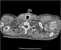
(c) CT 3 image

Fig.8. Results of Proposed Scheme

(d) CT 4 image

(a) CT 1 image

Fig.5. Results of Total Variation Denoising

(c) CT 3 image

(b) CT 2 image

(d) CT 4 image

Fig.6. Results of SURELET

(b) CT 2 image

(a) CT 1 image

(c) CT 3 image

Fig.7. Results of Bayes Thresholding

(d) CT 4 image

Table 2. PSNR of Denoised Images

	σ	TV method	SURELE T method	Bayes method	Proposed method
CT 1 image	10	32.14	33.25	31.50	33.39
	15	30.95	31.45	29.96	31.44
	20	29.45	30.10	28.21	30.05
	25	27.98	29.68	28.01	29.85
	30	26.31	28.47	27.25	28.54
	35	25.26	26.19	25.31	26.88
CT 2 image	10	31.54	32.12	30.98	32.47
	15	30.87	30.64	29.42	31.05
	20	28.95	29.08	28.47	29.53
	25	28.48	28.64	27.26	28.96
	30	27.69	28.03	26.17	28.11
	35	25.83	26.96	25.34	26.97
CT 3 image	10	32.33	33.19	31.98	33.89
	15	31.29	31.25	30.67	31.87
	20	29.84	30.98	28.68	30.91
	25	27.15	29.27	28.34	29.31
	30	26.29	28.54	27.52	28.67
	35	24.36	26.65	24.64	26.73
CT 4 image	10	32.65	33.65	31.63	33.79
	15	31.35	31.24	29.26	31.35
	20	29.64	30.19	28.31	30.61
	25	27.45	29.34	28.72	29.36
	30	26.64	28.21	27.37	28.42
	35	25.39	26.94	25.61	26.61

D. Comparisons

To validate the superiority of the proposed scheme, its performance is compared in terms of visual quality, PSNR, and Image Quality Index (IQI) of the denoised images using the various methods available in literature such as Total Variation (TV) (Goldstein et al. 2009), SURELET (Donoho et al. 1995) and Bayes methods (Abramovitch et al. 1998). In all the cases, db8 is used for wavelet decomposition and soft-thresholding is used to

The best values amongst all the methods are represented in bold. The results shown in tables demonstrate that in most of the cases, the proposed method is superior to all other methods. The results of TV denoising method as shown in fig. 5 gives edge preserved smooth denoised image but texture is not as good as for clinical purpose.

Table 3. IQI of Denoised Images

	σ	TV method	SURELE T method	Bayes method	Proposed method
CT 1 image	10	0.9931	0.9912	0.9924	0.9976
	15	0.9534	0.9856	0.9762	0.9865
	20	0.9312	0.9541	0.9365	0.9597
	25	0.8972	0.9165	0.9174	0.9248
	30	0.8903	0.8954	0.8832	0.8962
	35	0.8894	0.8762	0.8614	0.8747
CT 2 image	10	0.9817	0.9828	0.9751	0.9889
	15	0.9789	0.9794	0.9745	0.9831
	20	0.9421	0.9654	0.9241	0.9521
	25	0.8452	0.8684	0.8922	0.9047
	30	0.8364	0.8361	0.8632	0.8740
	35	0.8189	0.8314	0.8614	0.8694
CT 3 image	10	0.9874	0.9812	0.9914	0.9965
	15	0.9514	0.9614	0.9762	0.9893
	20	0.9423	0.9591	0.9432	0.9614
	25	0.9102	0.9241	0.9397	0.9235
	30	0.8964	0.8931	0.8942	0.9131
	35	0.8831	0.8894	0.8913	0.8941
CT 4 image	10	0.9871	0.9974	0.9954	0.9979
	15	0.9642	0.9831	0.9645	0.9846
	20	0.9409	0.9641	0.9469	0.9698
	25	0.9123	0.9352	0.9231	0.9411
	30	0.8991	0.8978	0.8945	0.9006
	35	0.8647	0.8649	0.8791	0.8771

• V. Conclusions

In this paper, a scheme is proposed based on locally patch thresholding, its method noise thresholding and aggregation. Due to selective patch sizes, the cost computation is reduced in compare of iterative methods.

The proposed scheme is taking the advantage of thresholding to denoised same pixel with different patch size. A gap in patch size is maintained by apply a rule to divide by 2 of previous patch size. A method noise with selective patch size may also help for more denoised and edge preserved patch. An aggregation scheme helps to provide a single final edge preserved and noise suppressed CT image. Final outcomes of proposed scheme are good in terms of noise suppression and edge preservation. All the results of proposed scheme are compared by existing methods. In most of the cases, the performance of proposed scheme is giving better values in terms of PSNR and IQI. Apart from performance metrics, the visual quality of proposed scheme over the CT images is also better in terms of clinically relevant details. Experimental results demonstrate that our proposed scheme: (i) effectively eliminate the noise in CT images, (ii) preserve the edge and structural information, and (iii) retain clinically relevant details.