A Novel Approach for MRI Brain Images Segmentation

Published Online March 2013 in MECS

The segmentation of Brain MR images to the different tissue such as white matter, gray matter and cerebrospinal fluid, is a topic of great importance and much research. MR brain images are widely used not only for detecting tissue deformities such as cancer and injuries but also for studying brain pathology [1]. In addition, many neurological diseases and conditions alter the normal volume and regional distribution of brain parenchyma (Gray and white matter), cerebrospinal fluid. Such abnormalities are commonly related to the conditions of hydrocephalus, cystic formation, brain atrophy and tumor growth. Manual segmentation of MR images is difficult, time consuming and costly. Errors can occur due to poor hand-eye coordination, low tissue contrast, unclear tissue boundaries caused by partial volumes and operator interpretation. Therefore, a highly accurate and robust tissue segmentation technique that provides systematic quantitative analysis of tissue volumes in brain MR images is became an important tool in many studies of neurodegenerative diseases. Extensive research has been already conducted to introduce new and more robust thresholding techniques [2]. Histogram-based thresholding is commonly known as a very popular tool in image segmentation. Here, the objective is to determine an efficient threshold for bilevel thresholding.

Image thresholding, which is a popular technique for image segmentation, is also regarded as an analytic image representation method [3]. It is computationally simpler than other existing algorithms, such as boundary detection [4, 5] or region dependent techniques [6, 7]. Its aim is to find an appropriate threshold for separating the object of interest from the background. The output of a thresholding process is a binary image where all pixels with gray levels higher than the determined threshold are classified as object and the rest of pixels are assigned to background, or vice versa.

Many approaches, including comprehensive overviews and comparative studies of image thresholding can be found in [8, 9, 10, 11]. Among these approaches, three of the most popular are Otsu's method [12], the minimum-error method [13, 14] and entropy based threshold method. Otsu method [12] can determine the threshold for image segmentation dynamically by maximizing the separability measures of the classes according to the image gray-level histogram. The minimum-error method ranked as the best in a comprehensive survey of image thresholding conducted by [2].

Qiao et al. [15] analyzed the limitation of thresholding methods based on within-class variance for images whose background and object have very different sizes and suggested a thresholding criterion based on the convex combination of within class variance and intensity contrast between the object and background. Recently Li Z, et al. [16] introduced another improvement for thresholding based on within-class variance and proposed a novel statistical criterion for threshold selection that takes class variance sum and variance discrepancy into account at the same time. Gamil and Abo-Eleneen proposed a thresholding method based on histogram projection by Fisher discriminate. This method is taken intensity contrast and within class variance into account at the same time [17].

Works on thresholding have utilized information theoretical approach in threshold's images. It constructs an optimization criterion based on the concept of entropy [18-20]. Sezgin and Sankur categorized the thresholding methods in six groups according to the information theory are exploiting [2]. One of these categories uses entropy as thresholding criteria. Generally these methods subdivided into entropic thresholding [21-24], cross-entropic thresholding [26] and fuzzy entropic thresholding [27].

The distribution of intensities in MR brain images is usually very complex, therefore, determining a threshold is difficult and most of the above mentioned thresholding methods fail. Mostly, thresholding method is combined with other methods [28]. The region growing method extends thresholding by combining it with connectivity. This technique needs seed for each region and has the same problem of thresholding for determining suitable threshold for homogeneity [29]. Clustering is the most popular method for medical image segmentation, with fuzzy c-means clustering and expectation– maximization algorithms being the typical methods, the applications of the expectation– maximization algorithm to brain image segmentation is reported in [30, 31]. A common disadvantage of expectation– maximization algorithms is that it is a supervised method and depends on the prior model and its parameters beside; the intensity distribution of brain images is modeled as a normal distribution, which is not the fact for noisy images. The fuzzy c-means clustering algorithm [32, 33] only considers intensity of image and in noisy images, intensity is not trustful. As a result, this algorithm does not produce a good result in noisy and in homogeneity images [32]. It has the drawback of increase in sensitivity of the membership function to noise. If MR image contains noise or is affected by artifacts, their presence can change the pixel intensities, which will result in an improper segmentation.

A second measure of disorder, besides entropy, exists which is called Fisher information measure (FI) [34] . The importance of this second type of “entropy” for the mathematical form of the laws of physics [34]. The

Fisher information is a measure of the fluctuations in the observations. In a sense, the Fisher information of an image specifies the quality of the image. The images contain a certain amount of Fisher information by which the highest precision, that is, the lowest variance, with which the structure parameters from these images can be estimated is established.

In this paper, a new thresholding method using the FI measure incorporate intensity contrast to segment medical images. It is the weighted sum of the Fisher information measure and intensity contrast between the object and background of the FI measure and intensity contrast between the object and background. The intensity contrast defined as the difference in mean intensities of the background and object. In this criterion, the FI within the two classes measures the intensity homogeneity within the object and background while intensity contrast captures the intensity difference between them. This method is useful in extracting objects of interest in images especially medical ones. Tests against a variety of brain MR images where the contrast is low or there is an overlap between modes, show that objects extracted successfully. The rest of this paper organized as follows: The Fisher information measure, related measures and the proposed threshold algorithm are presented in section II, the experimental results are presented in section III and the conclusions are presented in section 4.

• II.    FISHER INFORMATION MEASURE & RELATED MEASURES

In this section, the FI measure concept and related measures are reviewed. A new thresholding objective function and the corresponding algorithm are then proposed.

• A.    Fisher Information Measure

In statistics and information theory, the FI measure is thought of as the amount of information that an observable random variable carries about an unobservable parameter upon which the probability distribution of X depends. The Fisher information F ( θ ) can be written as [35]

F(θ) = -E(∂2logp(x;θ)) =E(∂logp(x;θ))2 (1) ∂θ2 ∂θ , where p(x;θ) is the probability density (mass) function for the random variable X.

The FI measure has applications in finding the variance of an estimator through the Cramer–Rao inequality, which states that the mean squared error of any estimate of a deterministic parameter has a lower bound known as Cramer–Rao lower bound [36]. Specifically, an intuitive interpretation behind the Fisher information is that it serves as a quantity, which determines the information of an observation X conveys with respect to estimating the parameter θ. Let the class of ‘‘unbiased’’ estimates, obeying the variance of such than estimator var(θˆ) obeys a relation [36].

var( θ ) ≥

1 F ( θ )

The special case of translation families deserves special mention. These are mono parametric families of distribution of the form f (x - θ) which are known up to the shift parameter θ All members of the family possess identical shape, and here FI measure adopts the appearance

_{I = (} d log f ( x ) ₎ 2 _{fdx =-} d ²log f ( x ) _{f ( x ) dx .                   (3)}

dx                   dx ²

This form of FI measure constitute the main ingredient of a powerful variational principal devised by Frieden [28], that gives rise to a substantial portion of the physics. In the consideration that follow we shall restrict ourselves to the form (3) of Fisher information measure.

• B.    Fisher Information Measure Versus Global Measures

Let X be a physical system that takes on a finite or accountably infinite number N of values that are characterized by the probability density p , i ∈ Ν where p is the probability of x and x ∈ (a, b) ⊆ ℜ, is assumed to be normalized to unity so

∑ N

p . In this case,

X can be specified by a probability vector, P = { p , p ..., p }. Its distribution over the interval (a; b) can be studied by using the following complementary spreading and information-theoretic measures: the FI measure [34] and the Shannon entropy [37]. The FI measure [34, 38, 39] and the Shannon entropy [36] of X are defined by the following respectively.

I ( X ) = ∑ i

( p ( x_{i + 1}) - p ( x_i ))² p ( x_i )

which follows from a suitable discretization of (2) and

H ( X ) = - ∑ p ( x_i ) log p ( x_i ).          (5)

i

These two quantities, which have a qualitatively different character, quantitatively measure the spreading of the random variable X in different and complementary ways. Shannon entropy H(X) uses uncertainty as a measure to describe the information that is contained in X. The sum in Eq. (5) can be taken in any order. Graphically, this scenario means that, if the curve p(x ) undergoes a rearrangement of its points ( x , p(x )), although the shape of the curve will drastically change the value of H remains constant. H is then said to be a global measure of the behavior of p(x ) . tails is not relevant, of course, when the tails fall of exponentially, which is the case for Gaussian or quasi-Gaussian distributions.

In contrast the Shannon entropy, the FI measure is very sensitive to the difference in the density at adjacent points of the variable. Indeed, when the density p(x ) undergoes a rearrangement of points x , although the shape of the density can change drastically the value of the entropy power remains constant according to Eq. (5),       however       the       local       slope values p(x ) - p(x ) change drastically and thus, the sum in Eq. (4), which defines the Fisher information, will also change substantially [34, 39].

The preceding discussion implies that the analytical properties of the Shannon entropy and the FI measures are quite different. Thus, whereas Shannon entropy is a global measure of smoothness in p ( x ) , FI is a local measure. Hence, when extremized through the variation of p ( x ) , Fisher’s form gives a differential equation whereas Shannon’s form always gives directly the same form of solution, an exponential function [34]. Therefore, if one of the two measures Shannon entropy (global) or FI (local) is to be used in a variation principle in order to derive the physical law p ( x ) describing a general scenario, a preference is given to the local measure, FI [34, 36]. For different applications of FI measure and more comparisons between the FI measure and information-theoretic measures we refer the reader to the book by Frieden [34].

• C.    The Proposed Threshold Algorithm

Let I denote a gray-scale image with L gray levels [0,1, ..., L - 1] . The number of pixels with gray level i is denoted by n and the total number of pixels by N = n + n + .... + n . The probability of gray level i appeared in the image is defined as:

n                L - 1

p_i = ⁱ , p_i ≥ 0, ∑ p_i = 1.

N             i = 0

Suppose the pixels in the image are divided into two classes A and B by a gray level, t. A is the set of pixels with levels [0,1, ..., t] , and the rest of pixels belong to B. A and B normally correspond to the object class and the back ground one, or vice versa. Then the probabilities of the two classes are given by p1  p2      pt

PA =     ,     ,....,, w1  w1

pt+1  pt+2

PB =       ,       ,....,, www where

t w1 (t ) = L Pi i = О and w2 (t) =1 — wx (k).

The mean gray levels of the two classes are defined as:

m_x ( t )   ^>2 ip i , w 2 ⁽ t ) = 1 ^— w i ^{( k} )

i = O and corresponding class variances are given by

__2    'S t —' ⁽ i - m i)² Pi

^ 1 = L ------- i = О

L^ (i — m2)2 Pi i = t + 1

The within-class variance, can be defined Otsu’s method [12]

^W = W1^2 + w^2,

Otsu selects a threshold t that minimizes the within-class variance 2 ; that is w t = arg, t < l min{ ^W}-

Kapur [23] has been employed the entropy criterion method in determining whether the optimal thresholding can provide a histogram based image segmentation with satisfactory desired characteristics. It selects a threshold t that maximizes the function.

f ( t ) = H a + H B ,

where

H.   >L ^Pi ln P^

i=о W1

and

Hb = L2P ln- i = t + 1 W2

The new method proposes FI as an optimality criterion as the following. The priori Fisher information for each distribution defined as.

t

S i = 1

F a ( t) = —

w ₁

⁽ p ⁽ x i + 1 ) ^— p ⁽ x i ⁾⁾² p ( x_i )

1      ( P ( x i + 1 ) — P ( x i ))²

^w 2 i = t + 1         P ⁽ xi )

The Fisher information F ( t ) is parametrically dependent upon the threshold value t for the foreground and background. We define the fisher information within the two classes as the following.

F ⁽ t ) = ⁽ w 1 F A ⁽ t ) + W 2 F B ⁽ t ))                    (9)

We propose a new criterion that combines the FI within the two classes and the intensity contrast,

J (a, t) = (1—a) F (t)—a(mx (t)—m2 (t ))2, where m (t) and m (t) are mean intensities of the object and background, respectively, F(t) is defined in Eq. (9). In this criterion, the FI within the two classes measures the intensity homogeneity within the object and background while intensity contrast captures the intensity difference between them. The parameter a is a weight that balances their contributions- When a = 1, the new criterion degenerates to the FI within the two classes. If a = 0 , thresholding is determined only by the intensity contrast, which may yield the threshold at the largest intensity of the image. Therefore, the weight should be in the range of ]0, 1[. The optimum threshold t * is selected by maximizing the new criterion,

J ( a , t * ) = max J ( a , t ).       (10)

t

Eq. (10) actually tries to increase the Fisher information within two classes and decrease the intensity contrast simultaneously. In this way, the intensity contrast becomes an explicit factor for determining the optimum threshold.

• D.    Algorithm

The proposed algorithm is a simple and effective thresholding method. It defines a new criterion based on the FI and intensity contrast corresponding to two thresholded classes, and determines the optimal threshold by maximizing the criterion. For the above image I with L gray levels, the process determining the optimal threshold t ^* in our method is as follows:

• (1)    Initialize Max to be infinite and t = О , where Max is the maximum value of J ( a , t ), t is the temporal gray level.

• (2)    Repeat steps 3–4, L times.

• (3)    Compute the value of the criterion

J ( _a , t ) corresponding to gray level t by Eq. (10).

• (4)    Compare J ( _a , t ) and Max , if

J ( a , t ) >  Max , then

Max = J ( a , t ), t * = t and t = t + 1 ; else, t = t + 1 .

• III. EXPERIMENTAL RESULTS

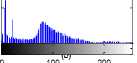
In this experiment, we implement threshold optimization method based on the Fisher information measure. To evaluate the performance of the proposed method, we apply it to a variety of MR brain images including normal axial, T2-weighted brain MRI slices, T1-weighted brain MR slices and glioma MR brain images. All of the images used are 256×256 and have 8-bit (i.e. 256 gray levels) types. The results from the proposed method compare with the most commonly used methods in the literature, namely Otsu’s method [14], Kapur’s method [22], MET [13].

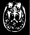
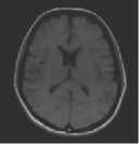
A. Normal MR Images

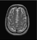
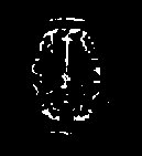
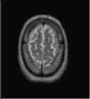
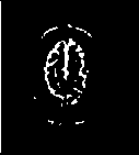
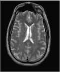
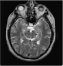
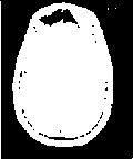
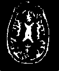
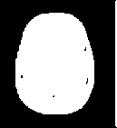
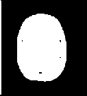
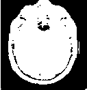
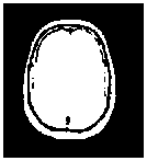
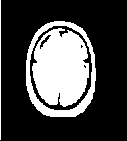
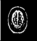
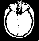
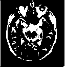
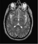
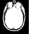
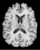
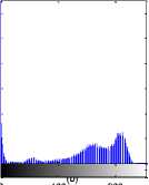
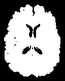
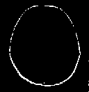
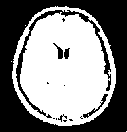
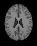
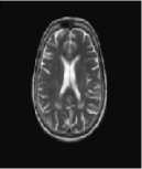
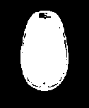
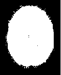
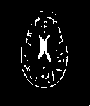
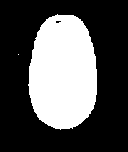
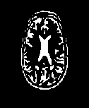
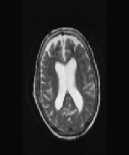
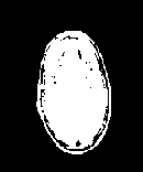
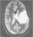
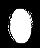
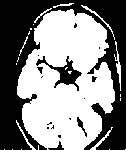
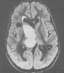
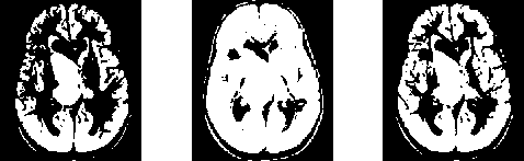
The first set of experiments are related to the segmentation of normal MR brain images. MR brain images contain the lateral ventricles, the interhemispheric fissure, Cortex, the gray matter and the white matter. The MR brain images segmentation facilitate in extracting these different brain tissues that helps in determining the volume of the tissues in threedimensional brain MR image, which yields in analyzing many neural disorders such as epilepsy and Alzheimer disease. In this study, a variety of MR brain images including T2-weighted brain MR slices and T1-weighted brain MRI slices. The original slices are displayed in Figs. 1-8 (a). The results yielded by the proposed method compared with the most commonly used methods in literature, Otsu’s method [12] Kapur’s method [23] and MET method [13]. Figs. 1-8 (f), show that the cortex and the ventricles are well extracted by the proposed method (i.e. different brain tissues) and showed its details in a clear way. Moreover, as can be seen in the segmented images in Figs. 1-8 (f), lesion or abnormal mass is not identified, and the ventricular system is not extensive and it is a median. Therefore, the image is a normal brain MR images. Otsu’s method (Figs. 1-8 (c)) extracted only the contour of the brain, the result of Kapur’s method and MET [13]are the worst (Figs. 1-8 (d) and (e)) All gray matter and white matter are misclassified, which is an unacceptable result.

(a)

(d)

(a)

(d)

(a)

(d)

(e)

(c)

(f)

(d)

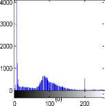
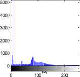
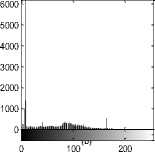
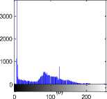
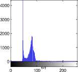
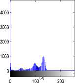
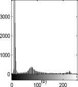
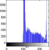
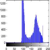
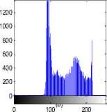
Fig.1. axial, T2-weighted MRI slice of human brain: (a) original, (b) histogram, (c) Otsu’smethod (d) Kapur, (e) MET (f) The proposed method with α = 0.04.

(e)

Fig.2. axial, T2-weighted MRI slice of human brain: (a) original, (b) histogram, (c) Otsu’smethod (d) Kapur, (e) MET (f) The proposed method with α = 0.025.

(e)

Fig.3. axial, T2-weighted MRI slice of human brain: (a) original, (b) histogram, (c) Otsu’smethod (d) Kapur, (e) MET (f) The proposed method with α = 0.65.

(e)

(c)

(f)

(f)

(c)

(f)

Fig.4. axial, T2-weighted MRI slice of human brain: (a) original, (b) histogram, (c) Otsu’smethod (d) Kapur, (e) MET (f) The proposed method with α = 0.007.

(a)

(c)

(a)

(c)

(d)

(e)

(f)

(d)

(e)                                                      (f)

(a)

Fig.5. axial, T2-weighted MRI slice of human brain: (a) original, (b) histogram, (c) Otsu’smethod (d) Kapur, (e) MET (f) The proposed method with α = 0.025.

(c)

Fig.8 T1-weighted MRI slice of human brain: (a) original, (b) histogram, (c) Otsu’smethod (d) Kapur, (e) MET (f) The proposed method with α = 0.0001.

(d)

(f)

B. Abnormal MR Images

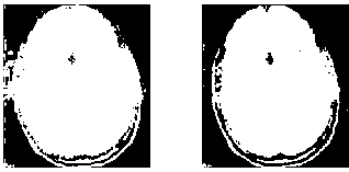
1) In this experiment two MR brain slices are used, one is sane MR brain image and the other is pathological MR brain image. The MR slices are displayed in Fig 9 (a) and Fig 10 (a). In this case, the goal of the segmentation is to quickly detect the different spaces and the white matter surrounding the ventricular space. The results yielded by the proposed method compared with, Otsu’s method [12] Kapur’s method [23] and MET [13]. Fig 9 (f) and Fig 10 (f), show that the cortex and the ventricles are well extracted by the proposed method. From these Figs. we notice that in the pathologic case , the modification of the size of the ventricle due to the atrophy is well extra

(a)

Fig.6 T1-weighted MRI slice of human brain: (a) original, (b) histogram, (c) Otsu’smethod (d) Kapur, (e) MET (f) The proposed method with α = 0.02.

(c)

(a)

(c)

(d)

(e)

(f)

(d)

(e)

(f)

Fig.7 T1-weighted MRI slice of human brain: (a) original, (b) histogram, (c) Otsu’smethod (d) Kapur, (e) MET (f) The proposed method with α = 0.0001.

Fig.9 axial, T2-weighted MRI slice of human brain: (a) original sane, (b) histogram, (c) Otsu’smethod (d) Kapur, (e) MET (f) The proposed method with α = 0.033.

(a)

(c)

(a)

(c)

(d)

(e)

(f)

(d)

(e)

(f)

Fig. 10 axial, T2-weighted MRI slice of human brain: (a) original pathology, (b) histogram, (c) Otsu’smethod (d) Kapur, (e) MET (f) The proposed method with α = 0.79.

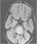
2) In this experiment three MR brain images with tumor (glioma ) are used [40]. The original MR brain images with tumor are displayed in Figs 1112 (a). Figs 11 to 12 (c, d, e, f ) demonstrate the results of segmentation of each images yielded by the proposed method, Otsu’s method [12] Kapur’s method [23] and MET [13]. Figs. 11-12 (f), show that the proposed method segmented MR brain images with tumor well and showed its details in a clear way.

(a)

Fig.12 T2-weighted MRI slice of human brain: (a) original, (b) histogram, (c) Otsu’smethod (d) Kapur, (e) MET (f) The proposed method with α = 0.0001.

(c)

(c)

(d)

(f)

(d)                                                      (e)                                                       (f)

Fig.11 T2-weighted MRI slice of human brain: (a) original, (b) histogram, (c) Otsu’smethod (d) Kapur, (e) MET (f) The proposed method with α = 0.0001.

Fig.13 T2-weighted MRI slice of human brain: (a) original, (b) histogram, (c) Otsu’smethod (d) Kapur, (e) MET (f) The proposed method with α = 0.0001.

IV. CONCLUSION AND PROSPECTS

Medical images generally contain unknown noise and considerable uncertainty, and therefore clinically acceptable segmentation performance is difficult to achieve. Probably, we will never find a super algorithm that can be successfully applied to all kinds of images. Therefore, it is appropriate to look for new techniques. The FI is a measure of the state of disorder of a system or phenomenon that makes it plays an important role in a physical theory. We have developed a simple but effective criterion for image segmentation that employs the combination between the FI measure and the intensity contrast. The underlying idea of the proposed method is to maximize the criterion. We applied the criterion on a normal MRI brain image and on a glioma MRI brain image. The results show that the method segments not only brain MR image without noise but also those with noise. The segmented normal and

glioma MRI brain images can be analyzed for diagnosis purpose. The proposed method has the following advantages:

• 1-    It characterized by its nonparametric and unsupervised nature of threshold selection.

• 2-    The implementation of the method is very simple.

ACKNOWLEDGMENT

The authors would like to express deep thanks to the referees for their helpful comments and suggestions which led to a considerable improvement in the presentation of this paper.

This research is supported by Qassim university under Grant SR-D-1258.