A Novel GRU Based Encoder-Decoder Model (GRUED) Using Inverse Distance Weighted Interpolation for Air Quality Forecasting

Air pollution is a global emergency in today’s time. A problem that started low but has now manifested itself into a giant mammoth that’s engulfing billions of lives worldwide. The latest report of WHO on air pollution states that 99% of the global population is exposed to harmful air pollution levels at some time in the year [1]. With almost all countries facing the brunt of pollution, India has some alarming figures with 22 out of 30 most polluted cities in the world present in India (World Air Quality Report, 2020). Within India, one of the most effected states that remains in constant headlines for its severe air pollution problem is the national capital, New Delhi. Infamously termed as the ‘Gas Chamber Capital of the world’, Delhi’s air quality has been severely deteriorating over the last decade (IQAir Monitoring, 2020). Factors contributing to this problem in India range from population explosion, urbanization, industrialization, and technological revolution. The causes are diversified. and their management requires significant time and planning. To begin with, knowing in advance about the upcoming air quality degradation is the first step in the direction of change.

To enforce preventative measures and least harm to living beings in advent of pollution, gauging the situation beforehand is an optimal approach. If it is known in advance that the air quality levels of a geography are going to take a serious dip, the situation can be handled. Accurate prediction of air pollution accommodates for timely implementation of prevention policies in case of alarming levels. The topic of air quality forecasts overlaps the disciplines of environmental as well as computer science. Early research in air quality forecasting utilized deterministic models of forecast such as dispersion models, WRF-Chem techniques, chemical modelling, etc. These were time consuming approaches which were heavily dependent on pollutant emission source data [4]. Due to these limitations, statistical modelling approaches that were faster and more data driven were brought into use. Techniques such as ARIMA, GARCH model, fuzzy networks were the next choice in air quality forecasting[5].

Air quality forecasts require modelling complex historical environmental data for predictions. The spatial-temporal nature of data involved requires analyzing intricate relationships. Artificial Intelligence-based approaches are best suited for this use case. The fast and complex data manipulation models have experimentally established efficiency in air quality forecasting [6]. AI approached like Deep Learning and Machine Learning have the most aptly suited models for air quality forecasting. Such models are land specific and must be customized for the geography in study. This study focusses on developing a custom air quality forecaster based on the GRU Encoder Decoder (GRUED) Model using Inverse Distance Weighted Interpolation for the geography of Delhi, India. Delhi has a recurrent problem of hazardous air pollution. This unique composition of techniques will be proven the most efficient than other counterpart approaches. The target geography for study will be Delhi as the city faces an acute and historic problem of air pollution. The data and model implementation are heavily influenced by the territorial and climatic properties of the target geography and is customized for the same. The air quality forecaster model is compared with conventional LSTM model to establish the efficiency and optimization status of our model.

2.    Literature Review

The deteriorating condition of air quality is a matter of concern, but the situation can be tackled by adept planning and forecasting. If accurate information about the upcoming quality of air is obtained in advance, measures can be taken to prevent the situation from worsening. This is where the discipline of Air Quality Forecasting in close conjuncture with Air Quality Monitoring helps aid the situation and provide timely information to control the situation. Air Quality Monitoring is a pre-requisite domain to Air Quality Forecasting as it records and provides all necessary historic and real-time data in the forecasting process. The domain of Air Quality Forecasting is an inter-disciplinary study that spans from the knowledge domain of environmental science to the implementation sphere of information technology. Environmental science gives a deep know-how of climatic and pollutant data properties, relationships, and dependencies. Whereas technology makes use of that data and develops forecasting software based on the best technical frameworks available. Since a long time, researchers and environmentalists have made remarkable developments in this arena and come up with innovative strategies for air quality forecasting. This is an ongoing arena of research because of the dynamic geographical properties and evolving complex nature of pollutants.

Air quality forecasting models can be broadly categorized into two major categories- knowledge-driven models and data-driven models [7]. Knowledge-driven models require relevant information of atmospheric science as they are highly focused on the physical and chemical properties of air pollutants. Data-driven models are based on statistical inferences and can find hidden relations amongst the pollutant data set. Some of the widely used techniques in statistical modelling were Multiple Linear Regression Models (MLR), Autoregressive Integrated Moving Average Models (ARIMA), Generalized Autoregressive Conditional Heteroskedasticity Models (GARCH), Grey Model (GM) and Artificial Intelligence Models, Fuzzy Networks (FN), etc. [8].

A recent study in China [9] focused on the best combination of feature selection and model for forecasting air quality in 74 cities of China. This study evaluates the best approach for air quality forecasting. The study revealed that although statistical models are much simpler, efficient, and faster than deterministic models, a hybrid approach is best suited for air quality forecasting [10]. There are several research that support these findings. A study of Turkey [11] developed an early warning and air quality monitoring system for China that concludes hybrid models and especially Elman Neural Networks have an advantage in time series predictions. In this study, the use of hybrid models is proven to be more efficient and that is the line of path adopted for the development of our custom air quality forecaster. An American study [12] combines hybrid and geostatic interpolation techniques with Machine Learning to forecast PM 2.5 constituent particles. The importance of meteorological parameters in forecasting process outshine in this study. [13] proposes a hybrid forecasting model using Ensemble Empirical Mode Decomposition, Gray Correlation Analysis and Back-propagation ANN for China. The sequence of techniques applied in this research is a good baseline for model development phases.

Study of air pollutants is a spatial-temporal domain as the atmosphere adheres to space and time characteristics. Recent research [14] have revealed that temporal characteristics land-use parameters that are important in air quality assessment studies. The features and characteristics of every geography are dependent on its location and there is no fit all solution for a given land-use. That is the reason why even if similar models are used in separate countries or cities, they need to be fine-tuned for the meteorological basis of a location. Another study, [15] investigated the impact of meteorological parameters on ultrafine Particulate Matter (PM1.0) in China. To predict pollutants, previous pollutant data is important alongside meteorological parameters. The nature of pollutants, neighboring areas and impact of land and occupation has a great deal on pollutant dispersion in the air. Land-use regression modelling is also a popular forecasting mechanism for fine-scale ambient air pollutant predictions [16]. Both the above-mentioned studies established the need for time series sensitive data analysis techniques in our custom model.

The target geography for this study is an Indian city, hence certain Indian research were also considered. In the initial research of Air Quality forecasting in India in 2011, a team of researchers at IIT Delhi, [17] developed a forecasting framework using Principal Component Regression (PCR) and Multiple Linear Regression (MLR) techniques. The framework forecasted RSPM, SPM, SO2 and NO2, the major pollutants of that time using a seasonal forecast model. [18] implemented various Machine Learning techniques such as Linear Regression, Random Forest Regression, Decision Tree Regression, Support Vector Regression, etc. and compared their forecasting efficiencies for air pollutants in Delhi. This study was one of the initial research projects that does not focus on the current complex pollutant evolution. The study of Air Quality Forecasting in Delhi has evolved from the use of Gaussian Dispersion and deterministic approaches to the latest trend in statistical modelling- Artificial Intelligence techniques. Artificial Intelligence is an umbrella term for a group of technological approaches that focus on data and produce faster, efficient, and self-tuning prediction results [19]. One of the most popular techniques in this bunch is Machine Learning that focuses on developing self-learning programming solutions that are efficient decision makers requiring least human intervention. Apart from land-use, satellite imaging and geographical spread also have an impact on land use studies in air quality forecasting.

An interesting sub-domain of Machine Learning in the form of Deep Learning has been used in specialized predictive and classification studies and is slowly gaining pace in acceptance. Deep learning models based on neural networks are a proven state of the art technique for spatial temporal data extraction and prediction. Time and again they have proven to be experimentally more efficient than conventional statistical and Machine Learning-based algorithms. Recurrent Neural Network (RNN) is an optimization of a cyclical loop addition on top of FFNN [20]. A recent study of Delhi [21], aimed at predicting pollutant concentrations of O 3 , PM 2.5 , NO and CO using the Long Short-Term Memory (LSTM) Model. Other Deep Learning Models such as Long Short-Term Memory Deep Model (LSTM) and Recurrent Neural Networks (RNN) have been extensively used for forecasting weather, precipitation, traffic predictions and air quality (T-Tsai et al. 2018). The prime advantage of these networks is that they work best on data having temporal properties and can hold knowledge of past relationships amongst data that heavily influence future predictions.

3.    Study area and data

The geography under consideration for this study is the National Capital of India, New Delhi. Delhi is one of the most polluted cities of India and the world. The reason for Delhi as a choice of geography for this study is its growing pollution menace and dire need for preventative measures. It is situated in the northern part of India between the latitudes of 28°-24’-17” and 28°-53’-00” North and longitudes of 76°-50’-24” and 77°-20’-37” East. Delhi is a high population density land that serves as a habitat to over 30 million people in 1,482 km2 area which makes it the second most populous city in the whole of India. Covered in the Northern plains, Delhi faces extreme seasonal climate throughout the year and wind directions facilitates particle suspension in the air [22]. The combination of humid subtropical and semi-arid climatic conditions give Delhi a plethora of climatic variations throughout the year. The wind patterns influenced by the south-western and western disturbances lock up the pollutant particles suspended in the air. The densely populated capital has extremely high volumes of vehicular transmission with more than 15 million registered vehicles (IQAir Monitoring, 2020). Delhi experiences extremely high air pollution levels in the winter months and they continue to influence the air quality in Delhi all throughout the year.

Experiments in this study are performed on data retrieved from three different AQI monitoring stations in Delhi based on pollution hotspots. The hotspot count in Delhi has increased from 13 to 150 in a span of one year from 2021 to 2022 (Delhi Government Identifies 150 Air Pollution Hotspots - The Hindu, n.d.). Every hotspot has a nearby government established AQI monitoring station that records meteorological and climate data in real time through IoT sensors. These monitoring stations are controlled by government authorities such as CPCB, DPCC, SAFAR and IMDB. Monitoring stations for data consumed in this study have been chosen based on their location. Anand Vihar MS is a traffic heavy junction, RK Puram MS is an industrial junction and Punjabi Bagh MS is a residential junction. Data was collected mainly under the classification of meteorological and air pollutants as they impact air quality forecast. Four air pollutants namely Sulphur Dioxide (SO 2 ), Nitrogen Dioxide (NO 2 ), Ozone (O 3 ) and Carbon Monoxide (CO) as well as 6 meteorological parameters namely RH, WS, WD, SR, AT and BP were considered. For each station 5 years (20152019) data was retrieved from the official website of Central Pollution Control Board, Delhi (CPCB) in the form of Comma Separated Values (CSV) files.

4.    Methodology

The proposed methodology detailed in this section contains all the techniques that are required to build our custom air quality forecaster. These components are the basic building blocks put together in Section 5, proposed GRUED model framework.

• A.    Inverse Distance Weighted Interpolation (IDW)

IDW is a spatial interpolation technique that is used to interpolate missing values of a variable with reference to a spatial context [24]. This technique is widely used in time series datasets as it gives weightage to time intervals in the data being considered. IDW can be used to estimate the value of an unsampled (unknown) point from amongst a set of sampled (known) points. The technique is based on the logic that points closer to the un-estimated value has a greater influence than those far away from it [25]. Being a weighted technique, the weight of the unsampled point is computed based on the Shepard’s rule. The rule states that to calculate the weight w_i of the i^th unsampled point, its Euclidian distance d ij from the nearest sampled point is considered. The power variable p controls the rate of decrease of weights. It implies that the greater the value of power variable, the more influence is exerted by proximal values. The value of p is by default 2. This value can be hyper tuned by minimizing the overall RMSE.

w t =                                                     (1)

^d ij

The value of the distance dij of a sampled point from the unsampled point can be calculated using the formula mentioned below.

d tj = J^(x t - % ; )² - ⁽У - У ; )²

Once all sampling point weights (wi) and values (xi) are received, the final weight of the unsampled point is computed as follows- z = i^=1Wl xt/^^t (3)

• B.    Gated Recurrent Units (GRU)

Recurrent Neural Networks (RNN) suffer from short term memory retention of scanned data which implies that while processing long data inputs, initial data may be lost by the network. Also, the vanishing gradient problem in backpropagation in RNN makes it difficult to update weights as the gradient shrinks a lot when propagated back in time [26]. Long-Short Term Memory Networks (LSTM) and Gated Recurrent Unit Networks (GRU) were RNN’s workaround to these problems. The control flow of these networks was like RNN, but their internal operations differed variedly. GRU combines the gate architecture in LSTM into lesser and more meaningful structure that efficiently manages the vanishing gradient problem of RNNs. GRU has lesser gates than LSTM and eliminates the concept of cell state altogether. The major functional advantage of a GRU over RNN and its variants was that the weights are smaller in GRU, and training and generalization of the model are attained faster through fewer tensor operations.

A Gated Recurrent Unit (GRU) Network has primarily two gates- an update gate (z) and a reset gate (r). The update gate determines the way the newer information in the network amalgamates with the memory from previous units and the reset gate makes the decision of which information to propagate and which to discard. Evolving from an RNN model, a GRU combines the input and forget gates in update gate and reset gate applies to past hidden state. The equations for the calculation of update gate (z_t ) and reset gate (r_t ) are given as follows. Sigmoid activation function (cr) squeezes the results between range 0 to 1. Weight metrices of the three gates are W, W_r and W, constants are represented as b_r , b_z and b_s , x_t is the input element, hf is the candidate hidden state since it still needs to incorporate the actions of the update gate, h - is the previous hidden state and h_t the output hidden state. Fig. 1 demonstrates the arrangement of a basic GRU unit. Multiple such GRU structures have been used in our stacked GRUED model.

z, = а(% Uz + hi-1 Wz + bz)(4)

rt = c(xt Ur + ht-1 Wr + br)(5)

hi' = 0tan^(Xi Us + (hi-1. r) Ws + bs)(6)

ht = (1-z) .ht-1 + z .hi(7)

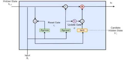
Fig. 1. A basic Gated Recurrent Unit component

• C.    The Encoder-Decoder Model

The Encoder-Decoder (ED) Model is a relatively new approach in Deep Learning but has been proven to deliver optimal results in time series forecasts. The ED model is often referred to as the Encoder-Decoder Sequence-to-Sequence Model as it focusses on processing an input sequence and generating another unrelated varying length output sequence [27]. This approach is especially beneficial when the input sequence has some relation flow with each other as in the case of timestamped or temporal data. The model components can hold and carry forward information about data and make future decisions based on past relationships or trends. These models are very popular in tasks like language translation, text summarization, image captioning, etc. [28].

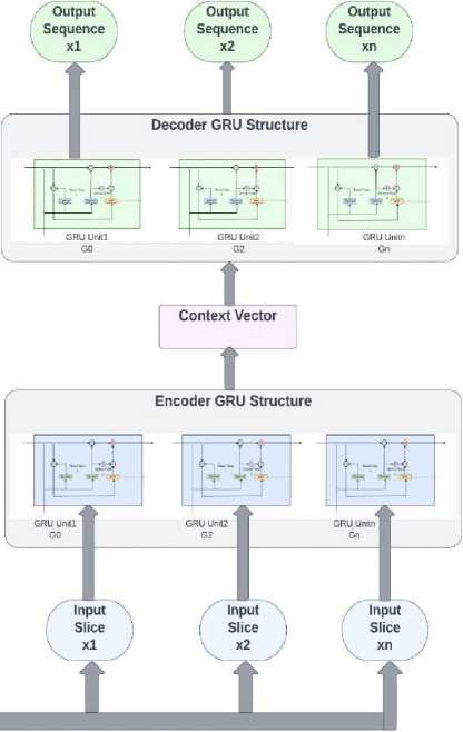
The Encoder-Decoder Model comprises of the Encoder and Decoder component that is based on multiple neural units of Recurrent Neural Network (RNN) and its variants such as Long-Short Term Memory Model (LSTM), Gated Recurrent Neural Network Model (GRU), Conventional Neural Network Model (CNN) etc. These individual deep units are stacked individually in the Encoder and Decoder component of the model. In this study, we have used Gated Recurrent Units as stacked components for our Encoder-Decoder model hence the proposed model is GRUED model. The units of the Encoder component process the input sequence in the vector representation and keep propagating it forward to consecutive units. It also intakes additional information about the input in the form of hidden states generated by the GRU units. Assuming that x = [x1, x2,x3 xt] is the input sequence, h = [h1, h2,h3.....ht] are the hidden layer states, the hidden states of the Encoder component are computed using the formula- ht = f(W(M) ht-1 + W(hz) xt)                                     (8)

Where ht is the hidden state of GRU component i, ht-1 is the previous hidden state for component i, xt is the input sequence representation of the ith component, f is the recurrent computation function of the GRU units. The Encoder compiles the information into a final context vector or intermediate vector, which is essentially a numerical array. The Encoder passes the same along with the final hidden state to the Decoder component [29]. The Decoder component then begins producing the output sequence, component by component. For this purpose, the Decoder also utilizes hidden states. The hidden state, ht for GRU unit i of the Decoder component are computed using the formula mentioned below- ht = g(W(h^ ht-1)                                           (9)

Where g is the activation function of the GRU unit. Hidden states in the Decoder component at a given instant are just a function of the hidden state of the previous component. The final output yt generated by each GRU unit t at a given time stamp is computed as- yt = softmax(Ws ht)                                    (10)

The final output of each GRU unit is computed using the weight of input at that unit W^s along with the hidden state h_t . The Softmax function generates a probability vector that is helpful towards the final output calculation. There are many variants to the conventional flow of this model. To avoid unnecessary focus on all information by the model, we can use the attention variant that refines the context vector to focus only on essential information [30]. Fig. 2 depicts below depicts the structure of an Encoder-Decoder unit.

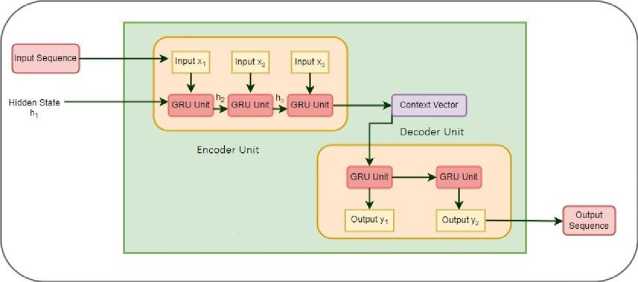
Fig. 2. An Encoder-Decoder Model Structure

5.    Proposed GRUED Model Framework

• A.    Preprocessing

  Development of the custom air quality forecaster was a two-phase process entailing data pre-processing and preparedness along with GRUED model development and fine tuning. Data required for this software was extracted from the CPCB’s portal for public access of historic meteorological and pollutant data. Data was assimilated from the portal over 5 years (2015-2019) and arranged in an orderly timestamped manner. Data was collected for each station of the three monitoring stations having 10 columns of meteorological and air pollutant segments in separate CSV files. Each monitoring station was studied separately and analyzed. In a single monitoring station case, each of the four pollutants to be predicted (SO 2 , NO 2 , O 3 , CO) were forecasted separately by changing the dependent and independent features for the model. Custom model training and fine tuning was applied in each case. The first step of pre-processing was feature engineering that was performed to extract essential and significant features that have maximum impact on predictions. Data visualizations were carried out to analyze the data from different dimensions and take data preprocessing decisions. In Fig. 3 shown below is the visualization of all pollutant data extracted from the CSV files. These line plots are indicative of the data distribution and help in studying the data gap, frequency, and missing data patterns. This data is of Anand Vihar monitoring station, and it shows that the frequency of missing data is erratic with huge gaps in between making interpolation techniques such as linear and polynomial unsuitable. Hence, we use a special interpolation technique for TS data such as Inverse Distance Weighted Interpolation. There is no regular pattern in data spikes and hence seasonality needs to be evaluated for time differencing.

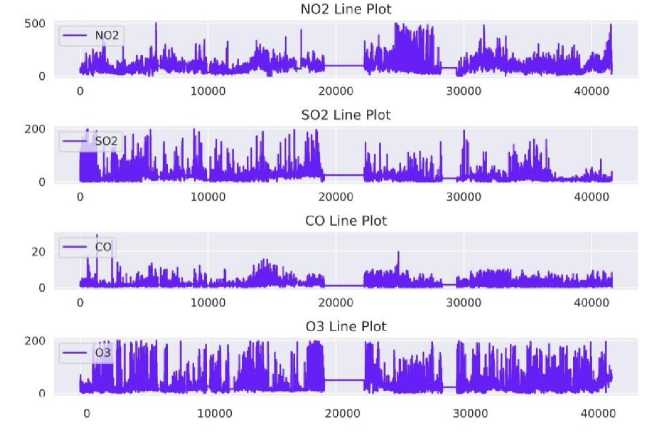
Fig. 3. Density plot visualization for data analysis segment

The next component for data pre-processing is plotting monthly, yearly, and seasonal data trends for pattern analysis in Fig. 3 and 4.

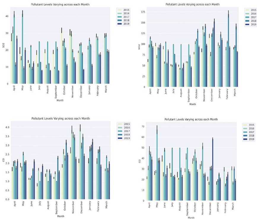
Fig. 4. Monthly air pollutant data pattern analysis

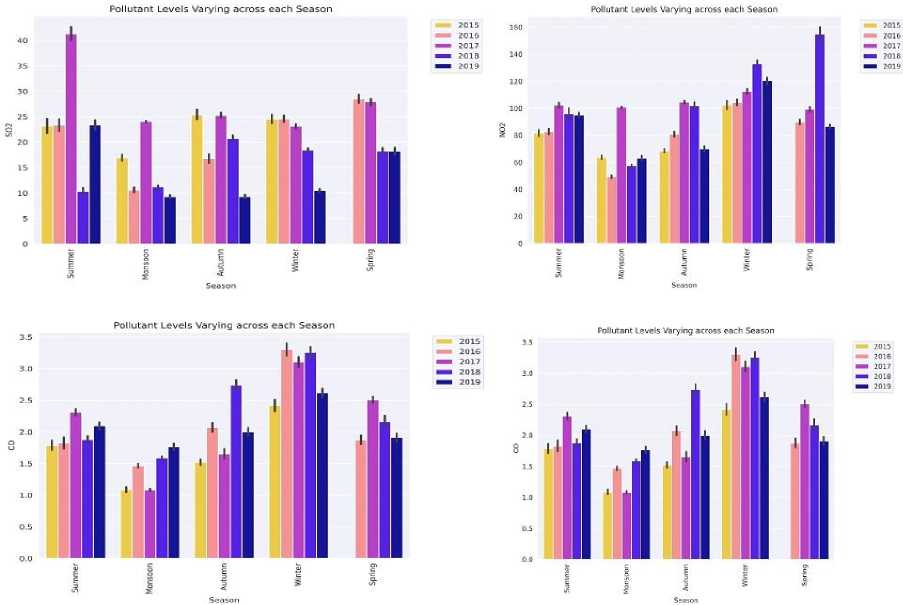
Fig. 5. Seasonal air pollutant data pattern analysis

The pattern analysis of data for Anand Vihar station reveals that the concentration for every pollutant is higher in the winter and the spring months. Seasons and time of the year have an impact on the pollution levels in Delhi. The onset of monsoon gets these levels on an all-time low throughout the year. The knowledge of the temporal nature of data helps fine tune a more sophisticated model. This information is critical to be remembered as a trend for our GRUED model. From this information it was clear to take the timestamp as a factor in pollutant prediction. After preprocessing begins the model building and fine-tuning phase. For the model building phase, the dataset is split into training and test data in the ratio 80:20 separately for every monitoring station. To bring the selected features to a uniform scale, standard scaling is performed on the dataset. Once the basic parameters of the model are set, the next phase is to segment the processed data into chunks/windows to be fed into the GRUED network. This is done using a window generator logic that is detailed in the next segment.

• B.    GRUED Model Window Generator

After the basic data pre-processing, the next phase is a simple GRU model creation and tuning that will be incorporated in the Encoder-Decoder architecture. Each of the tasks in model building segment are done using the basics of abstraction and encapsulation philosophies through separate classes and dedicated methods for performing individual tasks. The dataset under consideration is used in the formation of a window-generator object that forms data windows for inputs in the GRU network. A window object takes parameters as input width, label width and shift. Input width being the number of input features, label width as the number of labels to predict and shift as the time difference between the last input value and label to predict. Rolling mean values of all features are considered in this approach as they are more suitable for time series data.

We change the window parameters according to every pollutant in an individual model run and predict separately through the GRU network. In every pollutant prediction cycle, other highly co-related features are excluded from computation. The window object is formed by a window generator class that has functions to create the TensorFlow dataset from the data frame, separate the batch of TensorFlow dataset into input and label datasets and property allocation methods for ease of access. Using these window objects, the basic GRU model unit is compiled and tuned. Mean Absolute Error (MAE) is used as the loss function, metrics is calculated using Mean Squared Error (MSE) and call backs are used to stop the training process if loss value is not decreasing in consecutive epochs. With this the basics of model building phase are completed, and the next step is to fit in the individual GRU components into a stacked GRUED model. The next section details the building basics of the GRUED model proposed in this research.

• C.    The GRUED Model Architecture

Once a basic GRU unit is setup, individual GRU units are stacked up in the Encoder-Decoder setup. To set up the encoder and decoder GRUs, we begin with setting up the input tensor and dimension of the latent representation space called context. This is where the total window size and features are passed for the ED model. Context dimension also defines the number of GRU units in the encoder and decoder. The initial step is setting up the Encoder unit that takes number of GRU units i.e., 4 in this case, activation function as Rectified Linear Units (ReLU) in this case, return sequences that are hidden state tensors at each input time steps and return state that is the last state tensor. The final output of the last Encoder GRU is passed as a context sequence to the Decoder unit. The Decoder unit is initialized with number of GRU units i.e., 4 again, activation function as Rectified Linear Units (ReLU) and return sequence as True.

Once the Encoder and Decoder units are chained together all layers are grouped into a final GRUED model. The learning rate for this model is 0.02 and the optimizer used is Adam Optimizer. The model trains for 150 epochs and predicts one pollutant at a time. Evaluation metrices computed to gauge the model performance are Mean Squared Error (MSE), Mean Absolute Error (MAE), Root Mean Squared Error (RMSE) and Median Absolute Error (MedAE). Figure 6 mentioned below details the overall architecture of the GRUED model. Beginning from data extraction, compilation and pre-processing, data is further arranged in the window-based representation carried out through input slicing. These input slices are sequentially fed into the Encoder GRU network. The Encoder processes these inputs with additional information in the form of hidden states propagated between consecutive units. The encoder then compiles its intermediate transmission in the form of a context vector and passes to the Decoder GRU that sequentially outputs the desired sequence. In our case, the Decoder GRU will output 1 pollutant in 1 model run for every monitoring station. Fig 6. Drawn below is a comprehensive diagram of the proposed GRUED model framework.

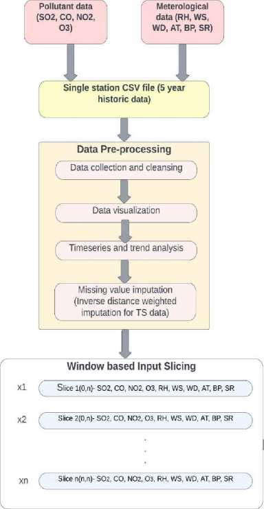
Fig. 6. The Proposed novel GRUED Model Framework for Air Quality Forecasting

6.    Experiments and Results

The set of experiments detailed above were run separately for three monitoring stations in Delhi namely- Anand Vihar MS, Punjabi Bagh MS and RK Puram MS in Delhi, India. These are a few of the monitoring stations set up by the government of NCT of Delhi for recording climatic parameters in real time through IoT devices. This climatic data is further available on public portals of the government for Research and Development. For every monitoring station, the model was run to predict each of the four pollutants under consideration- SO 2, NO 2 , O 3, CO. To establish the efficiency and novelty of our proposed GRUED model, the same data set was run on a basic Long-Short Term Memory model and the performance of the two was compared based on certain evaluation metrices. For every pollutant forecast the GRUED model was trained and individually customized to best fit the data. Historical data for five years was utilized to train and test the model. Once the model was trained, the forecasts were evaluated with actual observed values and efficiency was computed. The model performances were compared based on four evaluation metrics- MAE, MSE, RMSE and MedAE. Mean Absolute Error (MAE) was an outlier insensitive metrics that depicts the average error of absolute values. Root Mean Squared Error (RMSE) was a measure of the standard deviation of residual errors. Mean Squared Error (MSE) depicts the average of squared error values. Median Absolute Error (MedAE) considers missing values in averaging out errors of values under consideration. The formulae for computation of each of these metrics is mentioned below-

МАЕ = 1 ^₌i | X t - X i-I l

RMSE = Jz^J^-^2

mse = 1 z p=i ( X t - X t' )²

MedAE = median_n {| X_t - X_t' |}

Lesser error values indicate a more efficient forecasting model. GRUED model and a basic LSTM model are trained and run to forecast on the same historical data under consideration. The aim is to prove that our GRUED model has lesser error values for every evaluation metric for every pollutant forecast. Table 1, 2 and 3 mentioned above provide a sneak into the comparative analysis of the GRUED model and LSTM model. The three tables correspond to pollutant forecasts for three different datasets each of one monitoring station.

Table 1. Comparative prediction results for Anand Vihar Monitoring Station

Pollutant Predicted	Model Evaluated	Evaluation Metrics Comparison
		MAE	RMSE	MSE	MedAE
SO 2	LSTM	4.6642	8.8114	77.64	2.9465
	GRUED Model	2.9602	6.7211	45.1735	1.3649
CO	LSTM	0.6282	0.9058	0.8204	0.4564
	GRUED Model	0.5755	0.8728	0.7618	0.3837
NO 2	LSTM	18.7319	29.562	873.9144	12.2194
	GRUED Model	14.1761	22.6883	514.7591	9.2726
O 3	LSTM	10.5098	20.0212	400.8484	4.7674
	GRUED Model	8.4706	17.3246	300.1404	3.5324

Table 2. Comparative prediction results for Punjabi Bagh Monitoring Station

Pollutant Predicted	Model Evaluated	Evaluation Metrics Comparison
		MAE	RMSE	MSE	MedAE
SO 2	LSTM	4.9156	9.0919	82.6632	2.9852
	GRUED Model	3.3748	6.2037	38.4859	2.074
CO	LSTM	0.4762	0.6845	0.4686	0.359
	GRUED Model	0.3196	0.4876	0.2378	0.2157
NO 2	LSTM	10.5077	15.2923	233.8557	7.3414
	GRUED Model	8.3541	12.5967	158.677	5.6482
O 3	LSTM	7.9634	13.1839	173.8146	4.5448
	GRUED Model	5.2849	8.8964	79.146	3.0334

Table 3. Comparative prediction results for RK Puram Monitoring Station

Pollutant Predicted	Model Evaluated	Evaluation Metrics Comparison
		MAE	RMSE	MSE	MedAE
SO 2	LSTM	4.9038	6.7096	45.0192	3.7947
	GRUED Model	2.7365	4.391	19.2811	2.1133
CO	LSTM	0.4768	0.757	0.5731	0.2933
	GRUED Model	0.3884	0.6558	0.43	0.2145
NO 2	LSTM	10.6096	14.522	210.8892	8.2902
	GRUED Model	7.5028	11.368	129.2312	5.0748
O 3	LSTM	10.0992	16.8092	282.5485	5.6552
	GRUED Model	8.4561	14.0939	198.6377	4.561

For every station, meteorological historical five-year data has been considered. For every pollutant forecast, four evaluation metrics have been computed to determine the prediction error for GRUED model and LSTM model. GRUED model has lesser error rates in each pollutant forecast. Each prediction proves that the proposed GRUED model is more efficient and works better for all pollutants being forecasted. For Anand Vihar Monitoring Station, the GRUED model has MAE values 60.63%, 26.83%, 33.2%, 31.33% lower and RMSE values 43.4%, 19.5%, 26.4%, 27.7% lower than LSTM model. For Punjabi Bagh Monitoring Station, the GRUED model has MAE values 45.7%, 46.9%, 25.9%, 50.5% percent lower and RMSE values 46.6%, 38.7%, 21.3%, 48.3% lower than LSTM model. Finally, for RK Puram Monitoring Station, the GRUED model has MAE values 78.8%, 23.1%, 41.5%, 19.4% 52.5% lower and RMSE values 15.2%, 27.7%, 19.2% lower than LSTM model. The MSE and MedAE metrics also follow the same pattern. The GRUED model was very well fitted for all four pollutant predictions in each of the Monitoring Station. Fig. 7, 8 and 9 depict the well fitted model predictions for each monitoring station. Three different figures correspond to one Monitoring Station each. Each figure consists of four graphs. One graph represents a single pollutant forecast. The black lines are the actual pollutant concentrations, and the red lines are the model predictions. As evident, there is maximum overlap of the two types of values and the model best fits all values under prediction.

502 Cone

Fig. 7. Graphical representation of GRUED model predictions for Anand Vihar MS

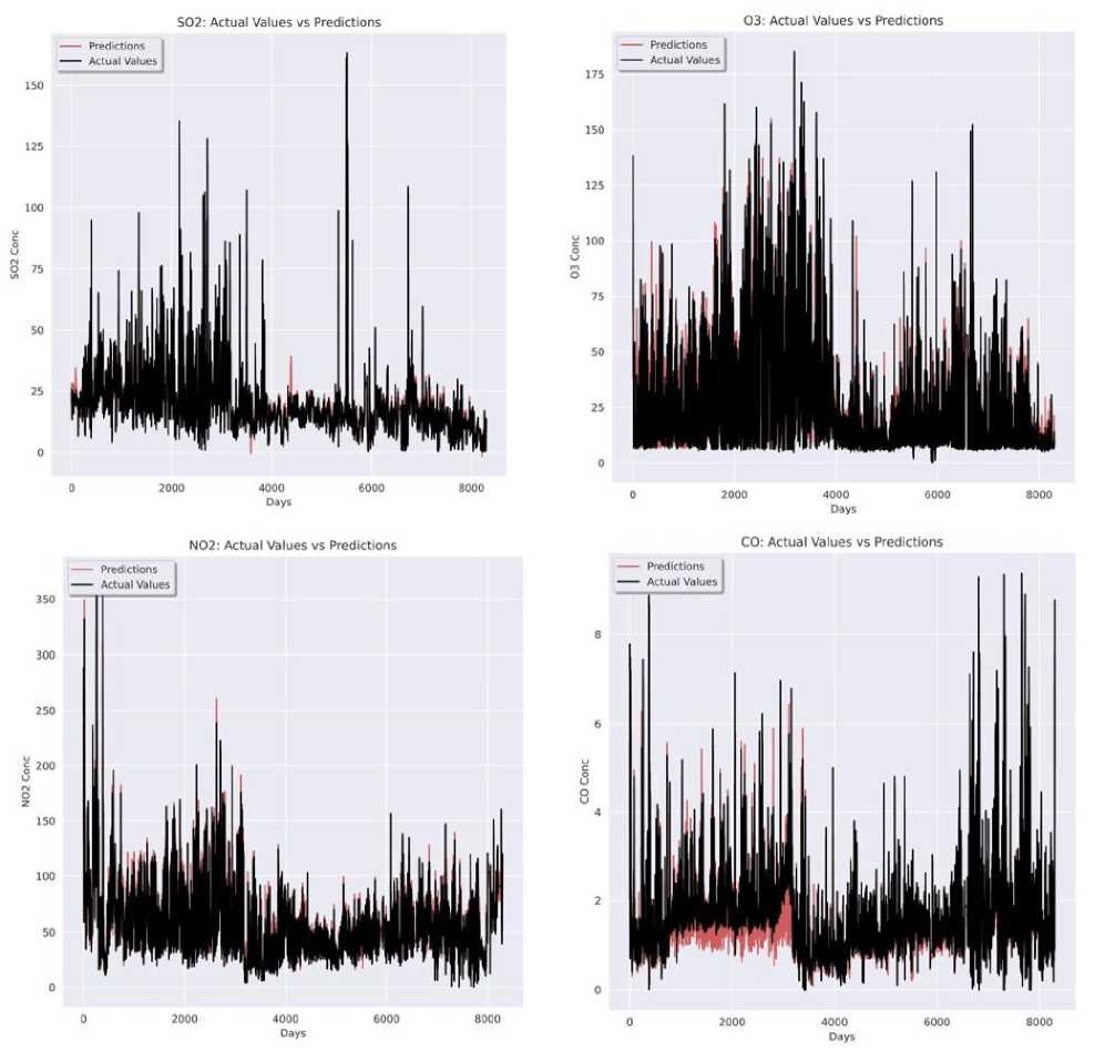
Fig. 8. Graphical representation of GRUED model predictions for Punjabi Bagh MS

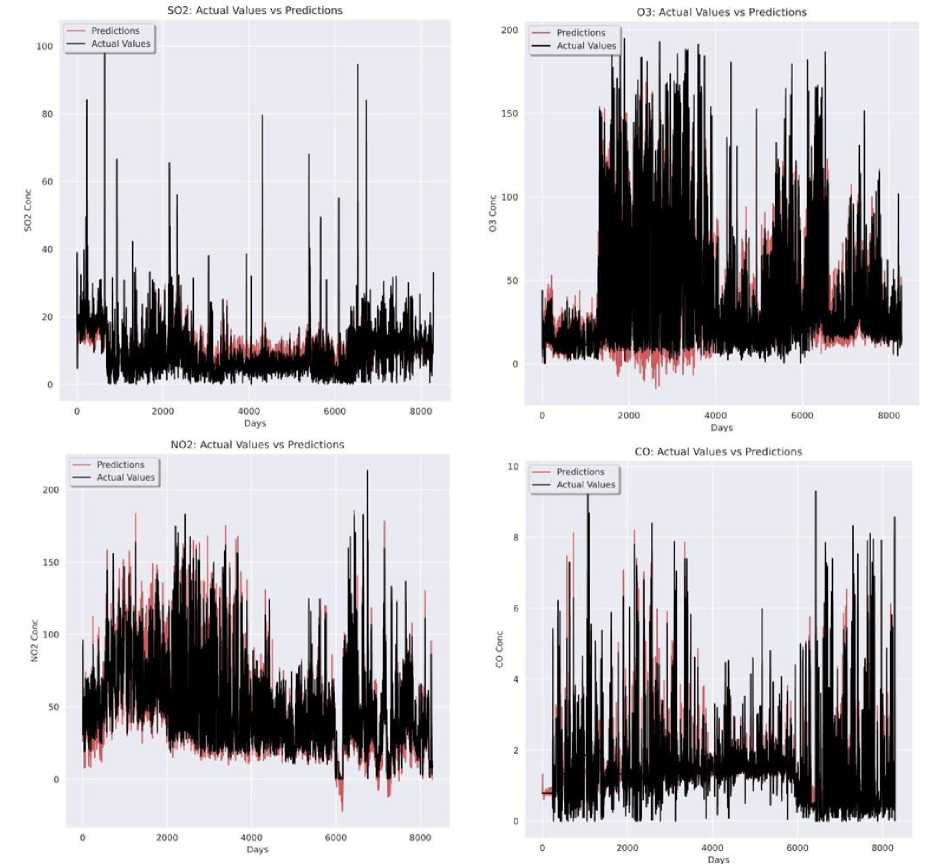
Fig. 9. Graphical representation of GRUED model predictions for RK Puram MS

7.    Conclusion

This study proposes a novel custom air quality forecaster to predict the pollutant concentrations for the city of Delhi, India. The novelty of this research lies in the combination of data processing techniques and GRU based Encoder-Decode (GRUED) architecture incorporated to predict the air quality data for Delhi. The combination of techniques and model efficiency is novel and more efficient than counterpart approaches. Timeseries forecasting has been an essential component of meteorological data-based research as it caters to the complex nature of data under consideration. The research also incorporates a unique interpolation technique in this approach called Inverse Distance Weighted Interpolation (IDW) that is especially designed to impute missing values for data that have a temporal component associated. The GRUED model proposed in this study makes use of stacked GRU components fitted in the Encoder-Decoder architecture. Experiments reveal that the custom GRUED model forecasts all air pollutants with greater efficiency and less error rates than the corresponding LSTM model. The performance efficiency of the custom model is performed by evaluation metrics such as MAE, RMSE, MSE and MedAE. The model is capable of forecasting single day as well as multi day advance pollutant concentrations. The GRUED model can be applied for air quality forecasting for Delhi, India as well as other geographies with some minor customizations. This model can also be used to forecast other meteorological parameters apart from pollutant concentrations.

The research utilizes historical data recorded by government portals and hence primary data collection is one main limitation of this study. Also, this study does not focus on the source of pollutant concentration rise that is a major component in improving air quality. Further the research can be extended by incorporating different air pollutants such as PM10, PM2.5, Benzene, Toluene, NO, etc. and meteorological parameters’ combination in the model. Also, other variants of the sequence-to-sequence architecture such as attention-based Encoder-Decoder model can be added to visualize the performance enhancements. Being a time series-based analysis, the study can be extended in other time series forecasting domains such as stock market predictions, weather condition forecasts, housing price predictions, COVID trend analysis, etc.