A novel hybrid method based on krill herd and cuckoo search for optimal power flow problem

The problem of optimal power flow (OPF) is significated considerable attention in recent years and has based its position among the main tools for the operation and planning of recent power systems. OPF is a nonlinear programming problem. The major objective is to find the correct adjustment of its control variables that optimize specific objective functions/functions while sufficient the operational constraints of equality and inequality at specified loading settings and defined system parameters [1-3].

The OPF has been applied to regulate the production of real powers, generators terminal voltages, setting of transformer taps, shunt reactors/capacitors and other control variables to improve the power system requirements by minimizing the production fuel costs, reducing the network active power losses, enhance the voltage stability and voltage profile at load buses. The previous requirements are achieved while all operational requirements are preserved within the accepted operation limitations as The voltages of load bus, the reactive power products of the generator, the network's power flows and whole other state variables in the power system within their assure and operational bounds.

In its most popular formulation, the OPF is static, a non-convex, wide-ranging optimization problem with both discontinuous and continuous control variables. Even in operating cost functions’ absence of non-convex generators, prohibited operating zones (POZ) of generating units and discontinuous control variables, the OPF problem is a non-convex because of the presence of non-linear alternating current power flow equality constraints. The existence of discontinuous control variables, like transformer tap positions, phase shifters, switchable shunt devices, added more difficulty the formulation and solution of the problem.

The methods were evolving to solve OPF problem can be categorized into two types conventional and advanced optimization techniques. The traditional optimization techniques were used derivatives and gradient operators. These techniques are usually not capable to find or determine the global optimal. Several mathematical suppositions like analytic, convex and differential objective functions must be made to simplicity the problem. Nevertheless, the OPF's problem is a problem of optimization non-convex and non-smooth objective function in general. As a result, it is significant to evolve optimization methods that are effective in dominating these disadvantages and to treat this hardness effectively. The computational materials’ evolution in recent decades has motivated to the development of advanced optimization methods that were so-called meta-heuristics.

These techniques can dominate many disadvantages of conventional techniques [4]. Several of these recent techniques have been applied to solve the OPF problem like: Simulated Annealing (SA) [5], Genetic Algorithm (GA) [6,7], Differential Evolution (DE) [8], Tabu Search (TS) [9], Imperialist Competitive Algorithm (ICA) [10], Particle Swarm Optimization (PSO) [11], adaptive real coded biogeography-based optimization (ARCBBO)[12], Biogeography Based Optimization (BBO) [13,14], multiphase search algorithm [15], Gbest guided artificial bee colony algorithm(Gbest-ABC) [16], Gravitational Search Algorithm (GSA) [17] , Artificial Bee Colony (ABC) [18], Multi-objective Grey Wolf Optimizer (MOGWO)[19], black-hole-based optimization (BHBO) [20], Teaching Learning based Optimization (TLBO) [21], Sine-Cosine Optimization algorithm (SCOA) [22], Group Search Optimization (GSO) [23], hybrid algorithm of particle swarm optimizer with grey wolves(PSO-GWO) [24], quasi-oppositional teaching–learning based optimization [31]have been incorporated into it. Meanwhile, many state-of-the-art meta-heuristic techniques, like Improved Colliding Bodies Optimization (ICBO) [32], Moth Swarm Algorithm (MSA) [33], MothFlame Optimization (MFO) [34], cuckoo search [35], firefly algorithm [36] and Backtracking Search Optimization Algorithm (BSA) [37] Surveys of different meta-heuristics used to solve the problem of OPF are offered in[25] The applications of these methods on different size systems lead to competitive results and therefore were favorable and encouraging for more study in this trend. Furthermore, because of the objectives’ contrast where various functions can be envisaged for modeling the OPF problem, of course not technique can be seen as the preferable in solving whole OPF problems. Hence, it is constantly needed to have a novel technique that can successfully solve several of the OPF problems.

Optimization is turning a area of request to analysts, particularly since a framework's the competence depends on obtaining an arrangement an order that can be acquired through suitable optimization technique. It is a method in order to discover the perfect solution next assessing the cost function that denotes the association among the system framework and its limitations. Presently, meta-heuristic algorithms are being formed in many regions for example crossbreeding, multi-objective type, binary type, preparing multi-layer perceptron and ways as Lévy flight, operator, and chaos theory. Most of these improvements happened because the deterministic and evolutionary components are used [23]. A perfect incorporation of global and local search has intensive local exploration and global exploration [25].

Krill herd method (KH) first suggested by Gandomi and Alavi in 2012 [26] and because it performs well, many optimization strategies such as chaotic theory [27, 28, 36], Flower Pollination Algorithm (FPA) [29] and colonial competitive differential evolution (CCDE)[30] have been hybridized with the fundamental KH algorithm as mutation operator with the objective of further enhancing the performance of KHA. Furthermore, to make KHA perform in the most ideal way, a parametric study has been conducted through an array of standard benchmark functions [38].

Furthermore, KHA is a new population-build swarm computation [26] in view of the Lagrangian and revolutionary conduct of krill people in wildlife for utilization and investigation in a problem of optimization. KH computation occasionally is not able to must avoid local optimum [27] and [28].

Firstly, as portrayed here, a successful hybrid Meta heuristic cuckoo search krill herd (CS-KHA) technique in light of KHA and CS is initially suggested to accelerate convergence. In CSKH, we use an essential KHA to select an encouraging solution set. Consequently, krill updating (KU) and krill abandoning (KA) operator started from CS algorithm are added to the method. The KU operator is to a decent encouraging arrangement; while KA operator is made use of further improving the investigation of the CS-KHA to substitute the worse krill's a small amount at the finale of every generation.

The performance of this approach is utilized to keep away from local optimum and obtain a worldwide ideal solution, in addition, minimal computational time to achieve the ideal solution, local minimum evasion, and quicker convergence, which produce them suitable for viable implementations for solving various constrained optimization problems. The purpose of this article is to develop an improved KHA called CS-KHA to solve OPF problem. So as to proven the evolution of the CS-KHA, its efficiencies are compared to CS, KHA and other well-known optimization methods.

The rest of article is structured in the next form: The following segment outlines the formulation of the OPF problem; meanwhile, section 3 depicts the algebraic equation of CS-KHA. Section 4 shows the simulation's results and discussion. While the finally conclusion of this paper is in section 5.

• II.    Formulation of optimal Power Flow (OPF)

The problem of OPF aims at finding the control variables’ optimal setting through minimizing /maximizing a predefined objective function while a collection of equality and inequality constraints satisfied. OPF considering the system's operating limit, hence it can be defined like a non-linear constrained optimization problem.

Minimize: f ( x , u )                (1)

Subject to:

h ( x , u ) = 0

g (x , u ) < 0                (2)

Where, и is the independent variable or control's vector, is the dependent variables or state's vector. Objective functions of OPF, g(x, и): set of inequality constraints, h(x, и): set of equality constraints.

• A.    Control variables

The vector of power network control variables is expressed as follows [37]:

u ^-[ P G 2 """ P G »_C ^,V G 1 """ ^V G „g , Q C 1 """ ^Q '    ^,T 1 """ T NT ]   ⁽³⁾

Where, p is the i-th active power bus generator. Chosen from bus 1 as swing bus is represented just and any one of the generator buses can be swing bus. V is the voltage magnitude at i-th voltage controlled generator bus, Tj is the j-th branch transformer tap, QCk is the shunt compensation at k-th bus. NG, NC and are the generators’ number, transformers and shunt VAR compensators. Any value within its range can be assumed as a control variable. Practically, transformer taps are not constant. Be that as it may, the tap settings indicated are in p.u. and outright voltage's estimation is not represented. Subsequently, for the aim of this study and to compare with previously described results, all control variables including tap settings are viewed constant for general cases of study.

• B.    State (dependent) variables

The power system's state variables can be expressed through vector x as:

G 1

Q_g is the generator's reactive power linked to bus i, is the p-th load bus's bus voltage (PQ bus) and Q-th line's line loading of is specified by. NL and nZ are the load buses’ number and lines of transmission respectively[40].

• C.    Power System Constraints

As aforesaid earlier, the problem of OPF presents both operational constraints on equality and inequality. These constraints are defined as follows:

C.1. Equality constraints

In OPF, the reactive and real power equilibrium equations are represented the system constraints of equality are formulated as for all system buses:

NB

Pg, — Pd, — V i D j [ ?« cos ( ^ ) + B j sin ( ^ _@ ) ] = 0   ⁽⁵⁾

j - 1

NB

Qg, — Qd, - V , Z V₇ G sin ( ^ ) + B j cos ( ^ ) ] - 0   ⁽⁶⁾

j - 1

Where, ^ - ^ — ^ is the voltage angles among bus i and bus j, NB is the buses’ number, Q and pm are reactive and real load demands. G is the transfer conductance and в is the susceptance among bus i and bus j, respectively.

C.2. Inequal ty constra nts

The inequality's constraint in the OPF reflects the equipment's operating limit in the power system, and too reflects the limitation of the line and the load bus to ensure the safety of the system.

• a)    Generator constraints:

V ™n < Vr < VrmaxVz e NG(7)

GGG

Pmin < PG < PmaxVi e NG(8)

Q < Qg, < QGmaxVie NG(9)

• b)    Transformer constraints:

T min <  T <  T max v j e NT j   jj

• c)    Shunt compensator constraints:

Qcmm < QCt < QcmaxVk e NC(11)

• d)    Security constraints:

Vmin < V, < V,maxVp e NL(12)

Lp       LpL

S < SmaxVq e nl(13)

l _q l _q

The control variables in constraints of inequality are self-limiting. The technique of optimization chooses a viable value for every like variable within the determined scope. Efficient methods for dealing with constraints of inequality related to dependent or state variables.

• III. Suggested Hybrid Technique

• A.    KH technique

The KH technique is built on the natural inspiration of conduct krill individuals’ imitation in the krill population. The KH technique is motivated by krill activities like [26]: 1/The movement of other krill individuals is induced; 2/Food search activity; 3/random scattering. The optimization technique has the ability to search for an uncertain search space.

• • Lagrangian model is extended to an n-dimensional decision space:

  dX^- - N _k + F_k + D_k dt

  
  
  
  

Where N the movement is stimulated by other members of the krill; F is the feeding movement and D is the physical diffusion of the k th krill.

The movement stimulated expresses the conservation of density through every individual. The matimatical formula reflects this conduct, which is worded as follows:

N'T = N max a_k + ^ n"

a — a local + a t arg ^et

Wherein Nmax is the highest stimulated velocity, o d indicates the inertia weight in [0, 1], N Ancient is the preceding movement alkcal and ajarget indicate the local effect of the neighbor, which is the best solution of the kth individual. atarget

is formulated by the following equations:

t arget        best ak    — C    K k best X k ,best

where, Cbest is the krill individual's effective coefficient with the preferable fitness for the first k krill, ˆ t             k,worst and Kˆ     are the worst and preferable krill's fitness value so far; is a random values’ number among 0 and 1. It is used to improve exploration, I is the current iterations’ number, and Imax is the iterations’ maximum number.

Foraging activities/movements are mathematically calculated as follows:

The foraging action consists of two major parameters. Premier is the position of the food F ^next , followed by the preceding experiment p around the position of the food.

^^next — V_f в + o F_k^revvous

P k — PT + вГ        (20)

Where, V _y is the foraging speed, o y is the foraging motion's inertia weight in the field [0, 1], F ^previous is the final foraging movement, p{^ood is the food attractive and РГ is the preferable fitness's effect of each krill. Depending on the foraging speed's measured values, take as 0.02 ( ms - 1 ).

D_k — D ^max 5

k

Wherein, D max is the highest induction velocity, 5 is the random direction vector [0, 1].

Lastly, the location of each krill is updated to:

X n^ext — X current + A x _k ( t )           (23)

A x ( t ) ^{— N}k ( t ) ^{+ F}k ( t ) ^{+ D}k ( t )       ⁽²⁴⁾

Where, t is the krill’s position.

• B.    Cuckoo search

Through optimizing the conduct of some cuckoo species, CS is suggested that is swarm intelligence's a type technique for optimization problems. In CS, Lévy flights are consolidated that decides the cuckoo's walking steps. For simplicity in portraying CS, Yang and Deb adopted some of the idealized rules. For instance, every cuckoo is just relating to one egg; the preferable nests would be preserved and not be obliterated; the possible host nest number is unchangeable, and an egg is recognized through the host bird with a possibility. In CS, every egg in a nest shows a solution. The CS is to take use of the recently created better solutions in place of a moderately poor solution. In this research, we just looked at every nest that merely had an egg. Thus, in this research, the difference between the nest egg and solution was not identified. The CS technique can make a good harmony between a local arbitrary walk and the irregular global exploratory walk using a switching parameter. The former one can be represented as

X * ^{+ 1} — X i + P s ® H ( P a - ^ ) ® ( X j - X k ) ⁽²⁵⁾

Where X t and X t are two various solutions choice jk at random, H(u) is function of a Heaviside , ε is a number of random drawn from a regular distribution, and sis the step size. For the global random walk, it is combined with Lévy flights as follows:

x ; ^{+ 1} — x ; + p l ( s , л ) , l ( s , л ) —

Я Г ( ^л ) sin ( ^^ )

v i -i- ;? ,^{( s} , ^s о ^ ⁰ ) n      s + л

Here, P >- 0 is the scaling factor of step size.

• C.    Proposed Hybrid CS-KHA procedure

To ameliorate the fundamental's the search capacity KH technique; genetic techniques are added to the method [26]. Numerical outcomes when contrast with other methods displays that KH II (only added crossover operator) performed the best.

In any case, KH can sometimes find it hard to come up with better solutions to several complicated problems. Consequently, in this article, a novel meta-heuristic technique by prompting KU operator and KA operator into KH to form a recent hybrid method, named CS-KHA is used to manage an OPF problem. The introduced KU/KA operators are roused by the authoritative CS algorithm. As such, in this paper, the property of cuckoo used in CS is supplemented to the krill to create excellent krill's a sort that can play out the KU/KA operator. The contrast amongst CSKH and KH is that the KU operator as a local search tool is used to adjust the new solution for every krill rather than rand walks used as KH's part (whereas in KH II, genetic generation techniques are employed). While KA operator is used to enhance further the exploration the method's ability by replacing some nests randomly thereby constructing new solutions. By the blending of CS and KH, CSKH can investigate the new search space with standard KH technique and KA operator and exploit the population information by KU operator. The main step of KU/KA operators used in CSKH method is presented by Algorithms 1 and 2, respectively.

Algorithm 1      KU operator

Begin

Get a krill i and update its solution using Lévy flights using Equation (25).

Evaluate its quality F

Select a krill j randomly.

If ( F ^F j )

Replace j with the novel solution and take the novel solution as X

Else

Update the position of krill using equation (22) as X end if

End.

Algorithm 2     KA operator

• 1.    Begin

K = rand ( NP , D )   p_a

.                                                                                                                      .

• 3   P i = P ; P 2 = P

• 4.    For i = 1 to ^NP (all krill) do.

• 6.    X = Xi + step OK (i,:);

• 7.    End for

• 8.    For i = I to ^NP (allkrill) do.

• 9.    If ^{F (} X^new ) ^F F ⁽ X i ) then

step = rand * ( Y. — Z. ) ;

.                                                                                                                    .

Firstly in the proposed method, standard KHA uses three movements to look for the best solutions and engage these movements to lead the candidate solutions for the following generation. In this, KU operator is then employed to carry out local search intensively to achieve better solutions. This operator can since it abuses the search space by Lévy flight. Towards the end of each generation, the KA operator is employed to additionally ameliorate the CS-KHA's the exploration by replacing the worse krill's a fraction (pa) .Along these lines, this component used in CS-KHA can completely extend the strong the KHA's exploration and gain overcome the absence of the KHA's weak exploitation . Above all, this technique can additional unwind the inconsistency among exploration and exploitation effectively. Furthermore, another basic change is the presentation of elitism scheme into the CSKH. Likewise, with other population-based methodologies, we employ a further focused elitism technique to hold the preferable solutions for the population. That elitism system forbids the preferable krill from existence demolished through three movements and KU/KA operator. By joining previously mentioned KU/KA operator and concentrated elitism design into unique KH technique to form a new CSKH algorithm (see Algorithm 3).

Algorithm 3     CSKH algorithm

Begin

Step 1: Initialization. Set the t =1,the population

P, V , D ^max,and N ^max , p and KEEP .

Step 2: Fitness evaluation.

Step 3: While t MaxGeneration do.

Sort the population.

Store the KEEP best krill.

^fori = 1: N_p (all krill) do

Perform the three motions .

Update the krill position by CU operator

(see Algorithm 1).

Evaluate each krill by X .

end for i

Destroy the worse krill and build new ones by

CA operator (see Algorithm 2).

Replace the KEEP worst krill with the KEEP best krill.

Sort the population.

• t = t + 1 .

Step 4: end while

End.

• IV. Objective functions and Studied Cases

A few contextual investigations with unique and multiobjective have been made for networks IEEE 30-bus, IEEE 57-bus and IEEE 118-bus test systems. The essential characteristics of this networks exam system are given in [33].

• A. IEEE 30 Bus system results

  A.1.Studied Cases

  A total of 8 studies of cases were implementing in the first exam system (IEEE 30-bus exam system). The first two cases studies reduced OPF's single objective function. The rest is multi-objective optimization, which translates into a single target with a weighting factor, as in numerous past studies and recreated here. The definitions of the studied cases are expressed as follows:

  • Case 1:    fuel cost's minimization

  This is the fundamental OPF's objective function in all studies. The relationship among fuel cost ($/h) and power generation Power (MW) is generally offered by two relationships, so the target function to be is reported as:

  NG

  f ( x , u ) = E a , - + b, PG_ + c i P G       ⁽²⁷⁾

  i = 1

  Where _a , b , c are the i-th generator's cost coefficients generating produce power. IEEE 30-bus system generators’ cost coefficients can be seen in [39].

  • Case 2:    fuel cost's minimization taking into account valve point effect

  The impact of the valve point should be taken into account for further practical and exact fuel cost function's modeling. The generating units with multi-valve steam turbines display a more prominent variety in the fuel-cost functions [32]. The valve loading multi-valve steam turbines’ impact is modeled as function of sinusoidal, which's the absolute value is added to the fundamental cost function. The steam plant's actual cost curve function becomes non-continuous. The aim of reducing fuel cost of generating with valve-point effect is presented by [40]:

  f ( x , u ) = E ( a , + b i P G i + c Д ) + dd, X sin ( e , x ( P m^{m -} P G ) )| ⁽²⁸⁾ i = 1

  Where, d and e are the coefficients that show the valve-point loading effect. The factors applied for calculations are given in [37].

  • Case 3:    Fuel cost's minimization and voltage stability enhancement

  Voltage dependability issues are accepting developing consideration in power systems as network breakdown have been experienced in last because of instability of voltage. Under normal condition and in the wakw of being subjected to unsettling influence, the power system's steadiness is portrayed through its capacity to keep up whole bus voltages in suitable boundaries. A system goes into voltage instability's a condition when an unsettling influence, augmentation in load demand or variation in system term causes a dynamic and wild abatement in voltage[14]. Systems with long lines of transmission and overwhelming loading are further inclined to the problem of voltage instability. In power system, a system's enhancing voltage stability is a vital

  
  

  part. Each bus's L-index fills in as perfect power system stability's marker [42]. The index's value can be between 0 and 1, where 0 existence the no load case whereas 1 is the voltage collapse. If a power system has NL load (PQ) buses’ number and NG generator (PV) buses’ number , L-index Lj's value of bus j is can be explained as:

  
  

  L j and

  
  

  NG

  ¹ - E F j,

  I = 1

  
  

  ^V

  V

  
  

  i

  
  

  j

  
  

  , where j = 1,2,

  
  

  F , =- [ Y ll Г1 Y lg ]

  
  

  ., NL

  
  
  
  

  Where, Y and Y sub-matrices and are gotten from YBUS system matrix next separating load (PQ) buses and generator (PV) buses as shown in (29).

  
  

  [ IL ~	=	Y LL	Y LG	"vl "	(30)
  L Ig _		L"gl	Ygl GL	_ Vg _

  
  

  ^L max = max ( ^Lj ) j = ^1,2......., ^{NL      (31)}

  The indicator L   varies among 0 and 1 where the

  max

  minimal the indicator, the further the system stable. Thus, enhancing voltage stability can be obtained by the reducing of L . Hence, the objective function can be formulated as:

  ( ng

  f ( x , u ) = | E ^a , + bi^P G,+ cP 1+ ^ L ^{X L} max   ⁽³²⁾

  V , = 1                         )

  
  

  Where, L_ma is chosen weight factor's value ^ is 100.

  Case 4: Fuel cost's m n m zat on and em ss on

  Electrical power's generation from traditional energy's sources releases dangerous gases for the environment. The nitrogen oxides (NOx) and sulfur oxides (SOx)'s amount and emission in tones per hr (t/h) is higher with augmented in generated power (in p.u. MW) next the relationship presented in Eq. (33).

  
  

  NB

  Emiss u)n = E | ( ^ + в Pg

  i =1^L                     ‘

  
  

  + y PI ) x 0.001 + ^ e ⁽ " ‘ P ^G- )

  
  
  
  

  Where, a , в , Y , ^ and ^i are all coefficients of emission provided in [41].

  Therefore, the objective function of this case is given by:

  NG

  f ( x , u ) = | E a , + bp + C/P1 1+ a x Emisk)n ⁽³⁴⁾

  
  

  The weight factors are chosen as = 100 in this case.

  
  

• Case 5:    fuel cost's minimization and voltage deviation

Deviation of voltage is voltage quality's a measure in the network. The deviation's index is too vital from the security part. The indicator is expressed as cumulative voltages deviation of whole load buses in the network from nominal unity's value. Mathematically it is formulated as:

(NL,

VD = IEК - 1 I

V p =1

The combining fuel cost's objective function and deviation of voltage is:

NG f (x , u ) = |E ai + b PG + c PG I + X/d xVD (36) V i =1               '

Where, factor of weight is give a value of 100 as in [32,33].

• Case 6:    Fuel cost minimization and active power loss

The power loss in system of transmission is certain because the lines have latent resistance. The active power loss to be reduced is formulated as:

nl     nl

P oss = Z E G V + V j - 2VУз cos ( ⁵ u ) ] ⁽³⁷⁾

i = 1 j = 1, j * i

A multi-objective case that aims at reducing fuel cost and active power loss simultaneously is transformed into single objective as:

NG f (x ,u ) = Eai + biPGi + CVG + Xp X Ploss  (38)

i = 1

Where, P is the active power loss and factor's value X is selection as 40.

• Case 7:    Fuel cost's minimization and voltage stability's enhancement

The objective function's formulation , comprising of both fuel cost taking into account the valve-point effect and voltage stability, this case's the objective function can be expressed as:

f (x ,u ) = £(a, + bP + c;p2 ) + i =1

Id,x(et X sin (Pgmm -Pgi))| + XL X L

The choice weight factor AL is too 100.

Case 8: fuel cost's minimization, emission, voltage deviation and losses

^{+ X} E ^X (40)

Four objectives are put together for this case study. Fuel cost, emission, voltage deviation and active power loss in the network are whole reduced together. The objective function is presented by:

(NG f (x ,u) = У^a. + b.P + c.P2

V i = 1

Emission + X VD x VD + X _p x P_loss

The weight factors are choice as in [33] with X = 19, Xq = 21 and X = 22 to balance between the objectives.

• V. Results and Discussion

  For optimizing's case 1 essential fuel cost, CS-KHA algorithms can produce to fuel costs of 799.0595 $/h which satisfies all the system constraints, complying to the vital constraints of inequality on generator reactive power, load bus voltage and line capacity . Amongst whole the constraints of inequality , constraint on load bus voltage was discovered to be vital as the load buses’ operating voltages are sometimes establish to be close the boundaries. Using the 3-methods (CS, KHA and CS-KHA), recent studies recorded better results when compared with present study are presented in table 2. The valve-point effect is studied for case 2 to achieve at a rise in cost than in case 1 with conclusive value of 830.0981$/h, get by CS-KHA. In a nutshell, in spite of the variation in efficiency is seen between three methods, produce one or more technique's outcome used in our work are better than most of the results revealed in past literatures on the problem of OPF are presented in table 2.

Case 3 to case 8 are for OPF with multi-objective for 30-bus system. In these case studies, the joined objective function's fitness is the significant factor in ranking the different optimization techniques’ outcome out. For a significant comparison, other techniques’ fitness value is calculated and provided here employing the different objective functions’ are weight factor. In multi-objective cases, an adjustment in weight factor e.g. elevated weight factor on fuel cost in case 3 the best values of both fuel cost and the system load buses’ Lmax , CS-KHA gives preferable produce of 799.5625 and 0.1251 respectively, superior to the other comparable algorithms as appears in the table 2. Two objectives of cost and emission are concurrently reduced in case 4 . Along with the fitness value, CS-KHA is at the cost and emission's least values in compared with in compared with other techniques presented in table 4.

Minimizing cost and voltage deviation (VD)'s in case 5, is achieved by CS-KHA which is the least among all other comparable techniques as appear in table 4.

In case 6 will reduce the cost and power loss. Table 3 shows’ quick review that any these techniques’ one or more CS, KHA and CS-KHA can give the preferable fitness values in whole the cases. Despite the fact that the preferable fitness is described by CS-KHA in case 6, a transitional value fuel cost, the forming objectives’ one,    minimum when compared with other methods as appears is accomplished. The active power loss's other goal is the    in table 4.

Convergence curve

Iteration

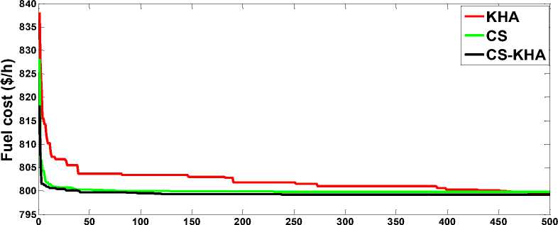
Fig.1. Convergent curves of Case 1

Table 1. The control variables’ optimal settings for Cases 1-3.

Case1             Case2             Case3

Control variable CS-KHA KHA CS    CS-KHA KHA CS   CS-KHA KHA CS

P G1 (MW)	177.7695	176.6985 177.0700		199.9957 199.9873 200.0000   178.3494 175.2915 178.5539
P G2 (MW)	48.8746	48.4488	48.8674	43.0739	42.5401	43.8734	48.2403	47.5274	48.9785
P G5 (MW)	21.0243	21.5532	21.3084	18.6343	19.1074	18.7891	20.5650	22.4648	21.3404
P G8 (MW)	21.5808	22.6989	21.0859	10.0300	10.0177	10.0000	20.3673	22.6681	21.5868
P G11 (MW)	10.8258	10.4866	11.8626	10.0000	10.0960	10.0000	12.7147	11.7468	10.0000
P G13 (MW)	12.0000	12.1911	12.0000	12.0000	12.0241	12.0000	12.0000	12.3124	12.0000

V 1 (p.u)	1.1000	1.1000	1.1000	1.1000	1.1000	1.1000	1.1000	1.1000  1.1000
V 2 (p.u)	1.0894	1.0891	1.1000	1.0854	1.0866	1.1000	1.0892	1.0937  1.0829
V 5 (p.u)	1.0634	1.0631	1.0728	1.0588	1.0583	1.1000	1.0665	1.0674  1.0513
V 8 (p.u)	1.0696	1.0708	1.0796	1.0665	1.0657	1.0878	1.0742	1.0825  1.0544
V 11 (p.u)	1.1000	1.1000	1.0957	1.1000	1.0985	1.1000	1.0999	1.0999  1.1000
V 13 (p.u)	1.1000	1.0944	1.1000	1.0975	1.0867	1.0160	1.1000	1.0982  1.1000
Qc 10( Mvar)	0.9873	0.7887	0	1.2012  0.3180  5.0000			4.8864  1	.6654  5.0000
Qc 12 (Mvar)	4.2959	0.8533	0	1.9153   0.1754 5.0000			0.7211	2.2254 5.0000
Qc 15 (Mvar)	3.0959	0.0015	5.0000	0.1687	0.0254	0	0.0187	0.9965         0
Qc17(Mvar)	5.0000	3.0633	5.0000	0.0310	0.0426	5.0000	0.6251	2.9405       0
Qc 20 (Mvar)	4.4733	3.4508	3.5533	5.0000	3.3646	5.0000	0.0525	0.0173  0.8864
Qc 21 (Mvar)	4.4607	0.4024	5.0000	0.1385	2.6324	5.0000	0.8977	0.3830  5.0000
Qc23(Mvar)	0.3577	1.9594	5.0000	2.1640	0.8609	5.0000	2.4613	0.1354       0
Qc 24 (Mvar)	5.0000	2.3827	5.0000	5.0000	1.2249	5.0000	4.0616	3.2836  5.0000
Qc 29 (Mvar)	3.4597	2.5427	5.0000	0.0572	2.9633	5.0000	0.3548	0.8722  5.0000

T 6–9        1.0315   1.0077   0.9718    1.0763   1.0090  1.1000    0.9910  0.9888  0.9000

T 6–10        0.9073   1.0210   1.1000    0.9027   1.0357  1.1000    0.9055  0.9503  1.1000

T 4–12        0.9875   1.0364   1.1000    1.0359   1.0579 0.9000    0.9696  0.9850  1.1000

T 28–27       0.9785   0.9963   1.0194    0.9805   1.0057  1.1000    0.9417  0.9446  0.9358

Fuel cost ($/h) 799.0595  799.4972 799.6547  830.0981 830.4199 833.5157  799.5625 799.8928 800.3034

VD      1.7638   1.1245   1.3088    1.2223  0.8337 0.9003    1.8465  1.7461  1.4380

Lmax     0.1290  0.1357  0.1350   0.1342  0.1393 0.1487    0.1251  0.1253  0.1268

Emission (ton/h) 0.3685  0.3653   0.3662   0.4425  0.4423 0.4424   0.3696  0.3608  0.3708

Ploss (MW) 8.6750  8.6771   8.7944   10.3339  10.3726 11.2625   8.8367  8.6110  9.0596

	Table 2. the results obtained are compared for Cases 1-3
Case 1	Case 2             Case 3
Algorithms	Fuel cost ($/h) Algorithms Fuel cost ($/h) Algorithms  Fuel cost($/h) Lmax
CS-KHA	799.0595    CS-KHA   830.0981     CS-KHA   799.5625   0.1251

KHA      799.497     KHA    830.4199     KHA     799.8928   0.1253

CS       799.6547     CS      833.5157     CS      800.3034   0.1268

BHBO[20] 799.921     BSA [37]  830.7779 Gbest-ABC [16] 801.5821   0.1370

ARCBBO [12] 800.5159 ICBO [32]  830.4531   MSA [33]   801.2248  0.13713

BSA[37] MSA[33] BBO[37]

799.0760    CBO[32]  830.473    BSA[37]    800.3340  0.1259 800.5099    ECBO[32] 830. 587   ICBO [32]   799.3277   0.1252 799.1267    DE[37]   830.4425   MDE [33]    802.0991   0.13744

Table 3. the control variables’ optimal settings for Cases 4-6.

Case4              Case5			ase6 KHA CS   CS-KHA KHA CS
Control variable CS-KHA KHA  CS		CS-KHA
P G1 (MW)	112.7779 112.9464 111.7271   176.2886 176.2432 177.5324  105.5625 105.3719 102.2213
P G2 (MW)	59.1035 58.7161 58.4399	49.1208 48.8217  49.1973   53.9578 52.9905  56.1303
P G5 (MW)	28.0892 28.1822 27.3951	21.3698 21.6226  21.7154   36.9416 37.0963 37.2408
P G8 (MW)	34.9991 35.0000 35.0000	22.0531 22.1836  22.8823   35.0000 34.9767  35.0000
P G11 (MW)	26.5804 27.1184 30.0000	12.4129 12.3589  10      29.9505 29.6778  30.0000
P G13 (MW)	26.9020 26.6188 26.2425	12     12	12      26.3434 27.7198  27.1722
V 1 (p.u)	1.1000  1.1000  1.1000	1.0387  1.0462	1.0442    1.1000  1.1000  1.1000
V 2 (p.u)	1.0928  1.0924  1.1000	1.0215  1.0295	1.0278    1.0930  1.0922   1.1000
V 5 (p.u)	1.0696  1.0688  1.0806	1.0092  1.0145	1.0155    1.0736  1.0695   1.0833
V 8 (p.u)	1.0798  1.0800  1.1000	1.0044  1.009	1.0035    1.0824  1.0802   1.1000
V 11 (p.u)	1.0992  1.0996  0.9000	1.0797  1.0241	1.0397    1.0997  1.0961   1.1000
V 13 (p.u)	1.1000  1.0900  1.1000	0.9844  0.9835	0.9967    1.1000  1.1000   1.1000
Qc 10( Mvar)	1.1530  1.1760  5.0000	0     5     5	1.5790  3.5805  5.0000
Qc 12 (Mvar)	3.3798  2.9034  5.0000	5     2.1588	0      3.0622  0.0852  0
Qc 15 (Mvar)	5.0000  1.5069  5.0000	4.9985  5	0      0.1757  4.1400  0
Qc 17 (Mvar)	3.7785  0.2768  5.0000	0    0.0767	0      5.0000  2.2509  0
Qc 20 (Mvar)	4.1506  1.0711  5.0000	5     5     5	5.0000  2.5827  5.0000
Qc21(Mvar)	1.1979  0.7196  5.0000	5     5     5	5.0000  3.6976  5.0000
Qc 23 (Mvar)	0.0935  0.9665  5.0000	4.9587  0	5      2.9975  0.0588  4.2787
Qc 24 (Mvar)	5.0000  0.2050  5.0000	5     5     5	5.0000  0.0048  5.0000
Qc29(Mvar)	1.4504  0.3080  5.0000	0    1.6478	5      2.2077  0.1971  2.1814
T 6–9	1.0603  1.0374  1.0772    1.0888  1.0403  1		.0596    1.0594   1.0402   1.1000
T 6–10	0.9000  0.9597 0.9000    0.9    0.9    0.9		0.9023  0.9182  0.9000
T 4–12	1.0186  1.0330 1.1000   0.9451  0.9228  0.9303    0.9945   1.0196  0.9966
T 28–27	0.9818  0.9857 1.1000   0	.9487  0.9613  1	0.9797   0.9856  0.9767  0.9910
Fuel cost ($/h)   835.3821 835.9164 839.0130  803.6357			803.6580 803.7306  853.1469 854.6579  857.3526
VD	1.6529  1.1912  0.8867    0.1045  0.1117		0.1066    1.8266   1.5253   1.8731
Lmax	0.1300  0.1342  0.1487   0.1468  0.1480		0.1490   0.1288  0.1310  0.1276
Emission (ton/h) 0.2421  0.2422  0.2404    0.3637  0.3635  0.3677   0.2317  0.2311   0.2287
Ploss (MW)	5.0521  5.1820  5.4047	9.8452  9.8300  9.9274    4.3558  4.4330   4.3646

Table 4. The results obtained are compared for Cases 4-6.

Case4              Case 5             Case 6

Algorithms Fuel cost ($/h) Emission (t/h) Algorithms Fuel cost ($/h) VD (pu) Algorithms Fuel cost($/h) Ploss(MW)

CS-KHA    835.3821   0.2421	CS-KHA 803.6357  0.1045   C	S-KHA 853.1469  4.3558
KHA     835.9164  0.2422     KHA    803.6580 0.1117   KHA		854.6579  4.4330
CS      839.0130   0.2404     CS     803.7306  0.1066    CS		857.3526   4.3646
BSA [37]  835.0199   0.2425	BHBO [20] 804.5975  0.1262	FPA [33] 859.1915  4.5404
GA-MPC[41] 835.0420   0.2423	BSA [37] 803.4294  0.1147	MSA [33] 855.2706  4.7981
MOGWO [19] 833.8528   0.2451	MSA[33] 803.3125 0.1084	MFO[33] 858.5812  4.5772
NSGA-II[19] 859.849   0.3214	MFO[33] 803.7911 0.1056

FPA[33]  803.6638 0.13659

Table 5. The control variables’ optimal settings for Cases 7 and 8.

Case 7                       Case 8

Control variable CS-KHA  KHA    CS      CS-KHA KHA    CS

P G1 (MW)	199.9573	200.0408  200.0001		122.7707  120.3378  121.4781
P G2 (MW)	44.0569	40.8348	47.1590	52.2425  53.9179  51.5677
P G5 (MW)	17.8443	18.9637	15.0000	31.2607  33.3589  30.5941
P G8 (MW)	10.0000	11.2088	10.0000	34.9961  35.0000  35.0000
P G11 (MW)	10.0028	10.5532	10.0000	26.4475  22.7272  30.0000
P G13 (MW)	12.0214	12.0000	12.0000	21.1133  23.4242  20.1360
V 1 (p.u)	1.1000	1.1000	1.1000	1.0999   1.1000	1.1000
V 2 (p.u)	1.0906	1.0880	1.1000	1.0890   1.0879	1.0887
V 5 (p.u)	1.0697	1.0665	1.0747	1.0627   1.0630	1.0636
V 8 (p.u)	1.0800	1.0752	1.0837	1.0718   1.0708	1.0733
V 11 (p.u)	1.0989	1.0995	1.1000	1.0560   1.0933	1.0206
V 13 (p.u)	1.1000	1.1000	1.1000	1.0325   1.0357	1.0562
Qc 10( Mvar)	0     4.8665   5.0000			2.5177   0.9657	0
Qc12(Mvar)	4.8593	0.1190	0	0.1353   2.0934	0
Qc 15 (Mvar)	3.5759	3.0433	5.0000	4.8952   1.4256	0
Qc 17 (Mvar)	4.6437	2.8878	0	3.2609   0.0210	5.0000
Qc20(Mvar)	2.5235	4.7887	0	5.0000   3.0301	5.0000
Qc 21 (Mvar)	0.0014	4.7253	0	0.1410   2.2403	5.0000
Qc 23 (Mvar)	4.2770	4.0181	5.0000	4.7800   0.0133	0
Qc24(Mvar)	0.2174	2.1304	5.0000	0.0437   0.4552	0
Qc 29 (Mvar)	0.6333	2.9869	0	0.5568   0.8862	5.0000
T 6–9	0.9844   1.0277    1.1000			1.0996   1.0405	1.1000

T 6–10	0.9000	0.9057	0.9000	0.9766	1.0636	0.9523
T 4–12	0.9658	0.9706	0.9919	1.0791	1.0482	1.1000
T 28–27	0.9469	0.9567	0.9472	1.0144	1.0126	1.0328

Fuel cost ($/h)   830.5273   830.3209  831.7243     828.8532  832.1724  831.1796

VD        1.9815    1.9553   1.7393       0.4827   0.5205   0.5015

Lmax        0.1248   0.1253   0.1253        0.1446   0.1440   0.1450

Emission (ton/h) 0.4426    0.4422   0.4437        0.2537  0.2508    0.2517

Ploss (MW)    10.4828   10.2013   10.7591       5.4308  5.3660    5.3759

Table 6. The results obtained are compared for Cases 7 and 8.

Case 7

Case 8

Algorithms Fuel cost($/h) Lmax           Algorithms Fuel cost($/h) Ploss (MW) VD(p.u) Emission (ton/h)

CS-KHA 830.5273  0.1248      CS-KHA   828.8532  5.4308  0.4827  0.2537

KHA 830.3209  0.1253      KHA     832.1724 5.3660  0.5205  0.2508

CS      831.7243  0.1253       CS      831.1796 5.3759  0.5015  0.2517

BSA [37]  832.7029  0.1262     FPA [33]  835.3699 5.5153  0.49969 0.24781

MSA [33]  830.639  5.6219  0.29385 0.25258

MFO[33]  830.9135 5.5971  0.33164 0.2523

MDE[33]  829.0942 6.0569  0.30347 0.2575

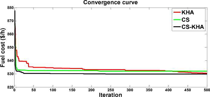
Fig.2. Convergent curves of Case 2

Important amelioration in fuel cost seen (through CS-KHA) in case 7's for multi-objective optimization where both cost considering the valve-point effect and L-max are minimized. Preferable to the other comparable algorithms as appears in table 6.

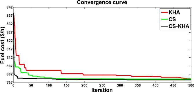
Cost, real power loss, emission and voltage deviation concurrently reduced four objectives are in case 8. Along with the fitness value, CS-KHA is at the cost and loss's least values in contrast with MSA [33] and FPA [33], as shown in Table 6. Graphical comparison the convergence of three proposed techniques for Case 1 and Case 2 of the objective functions related to the fuel cost is shown in Figures 1 and 2 respectively. The convergence speeds are Not distinctly various between the techniques. Be that as it may, fast and surprising convergence is seen for both KHA and CS-KHA during the search process's first phase. KHA converges to the ideal solution more consistently. Two-objective cases’ convergences are given in Fig.3. (3.a and 3.b), Fig. 4. and Fig. 5. (5.a and 5.b). For clarity, only one technique's convergence achieving optimal fitness value is shown in the graph.

Comparison among CS, KHA and CS- KHA

Table 7. Shows the statistical summary of 30 runs using three proposed algorithm as the fundamental search technique for each study carried out. The columns denote the best, worst, average and standard deviation values of the objective function in every case. It is clear that no single technique is capable to issue the best mean values in whole the cases. CS-KHA is found to be superior to KHA and CS in all cases for 30-bus and 57-bus system.

• A.    Results of IEEE 57-bus test system

So as to exam the usability of the suggested CS-KHA technique, a greater test system is take into account in this article, which is the IEEE 57-bus test system. 57-bus system's general system data are given in [43].

CASE 9: fuel cost minimization

The goal of this case is to reduce the total generating fuel cost. Hence, this case's the objective function is presented by (27). The CS-KHA is implementation so as to get the optimal settings for this case and the gained results are presented in Table 8. In this case minimizing the fuel cost's fundamental objective produce to a value of 41660.2273 $/h by CS-KHA, the most minimal when compared with other recent studies’ substantial results as seen in Table 9.

CASE 10: Fuel cost minimization and voltage deviation

The purpose of the objective function is to reduce simultaneously both fuel cost and voltage deviation. The transformed single objective function next equation (36)

with weight factor λ is chosen as 100. The results of such optimization using the suggested CS-KHA technique are given in Table 8. This table shows that the VD has been decrease from (1.5991 p.u.) to (0.6940 p.u.) compared with CASE 9. Hence, the cost has slightly augmented from (41660.2273 $/h) to (41712 $/h) compared with CASE 9.

• B.    Results of IEEE 118-bus test system:

CASE 11: Fuel cost minimization

To prove performance of the suggested hybrid CS-KHA, the large-scale IEEE 118-bus system is deliberated for study goal, the essential characteristics are presented in [43]. In general, the efficiency of the proposed algorithm is excellent for variables’ higher number in constrained optimization problems. Therefore, CS-KHA method is utilized to the system to decrease fuel cost. Hence, this case's objective function is presented by (27). The CS-KHA is implemented so as to get the optimal settings for this case and the gained results are presented in Table10. In this case, minimizing the fuel cost's fundamental objective produce to a value of 135260.45$/h by CS-KHA, the most minimal when compared with other recent studies’ substantial results as seen in Table 11.

• VI. Conclusion

In present study, a new Meta hybrid heuristic CSKH technique has been suggested to solve the problem of OPF. By merging the merits KU/KA operator of CS technique with the KH technique. Hence, the KH is improved and the CSKH algorithm is evaluated numerically.

The detailed expression of a new variant of KH algorithm is given, and the KU operator is adjusted dynamically in KU process. In the proposed hybrid CSKHA, a greedy option was used, often surpassing the standard CS and KH. Moreover, so as to more ameliorate the CSKH's exploration, each generation of end KA operators will be a small number of poor krill thrown away, and replaced by new randomly generated krill. The problem of OPF has been expressed as a constrained optimization problem where many objective functions have been taking into account to decrease the fuel cost, to enhance the voltage stability and to improve the voltage profile. However, non-smooth piece-wise quadratic cost objective function has been deliberated. The feasibility of the suggested CS-KHA technique for solving problems of OPF is confirm by apply three standard test power systems. The results of the simulation prove the success and robustness of the suggested method to solve problem of OPF in small and large test systems. In addition, the suggested methods in this study achieve significantly better than several other equivalent optimization techniques in obtaining solutions of OPF. Decrease in hourly operation cost has been based almost in whole the cases studied in the context of this literature. In order to add more complex objectives function when solving OPF problems, no method is the best way to solve all OPF problems. Therefore, there is always a require for a new method, capable of successfully solving as many OPF problems as possible. However, increased capability is often achieved by hybridizing method and deterministic optimization techniques. In the future, different settings of optimization techniques used in this article are chosen by trial and error to improve convergence characteristics and these settings can be optimized for improved effectiveness. Various types of sources energy, like solar cells, wind turbines can be involved in solving OPF problems.

a. Fuel cost

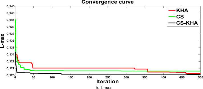
Fig.3. Convergent curves of Cas3 (bi-objectives)

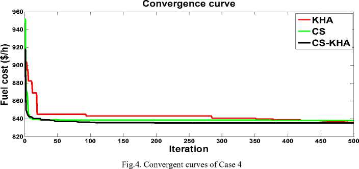
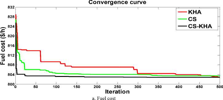
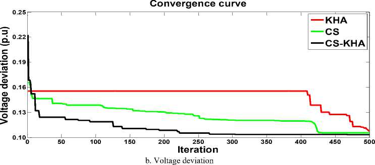
Fig.5. Convergent curves of the objectives of Case 5

Table 7. Summary of statistical indices of the CS-KHA with CS, KHA for Cases 1-10

CS-KHA             KHACS

Cace1 799.0595 799.4923 799.1761 0.0023  799.4972 799.9512 799.7572 0.024  799.6547 800.1054 799.9513.0321

Case2 830.0981 830.6713 830.1625 0.019  830.4199 830.9922 830.6918 0.033  833.5157 833.9145  833.73270.029

Case3 799.5625 799.8921 799.7005 0.03  799.8928 800.41   800.1367 0.043  800.3034 800.9133  800.6723 0.0352

Case4 835.3821 835.8811  835.5920 0.0015 835.9164 836.5764 836.2321 0.0191  839.0130 839.7700 839.32050.027

Case5 803.6357 803.980  803.8100 0.023  803.6580 804.2104 803.9683 0.03202 803.7306 804.2710  803.9360 0.0331

Case6 853.1469 853.5361  853.2742 0.0026  854.6579 855.3519 854.9914 0.041   857.3526 857.9720  857.6437 0.03602

Case7 830.5273 830.9407 830.7204 0.0031  830.3209 830.9859 830.7303 0.0342  831.7243 832.1926  831.9751 0.0284

Case8 828.8532 829.2302 828.9712 0.038  832.1724 832.8743  832.5126 0.0375 831.1796 831.6991  831.4425 0.0223

Case9 41660.2273 41660.840 41660.5703 0.04  41673.5922 41674.110 41673.9078 0.051  41717.8801 41718.4713 41718.0721 0.043

Case10 41712  41712.7701 41712.3923 0.062 41705  41705. 6203 41705.274 0.0421 41791  41791.8912 41791. 4822 .037

Table 8. The control variables’ optimal settings for Cases 9 and 10.

Control variable CS-KH		Case 9 KHA	CS	CS-KHA	Case 10 KHA	CS
P G1 (MW)	143.4297	145.0358	140.9221	140.6795	141.9955	146.9150
P G2 (MW)	87.0645	98.1294	77.7157	94.9802	92.1514	100.0000
P G3 (MW)	45.1917	47.2053	40.0000	47.1461	45.7668	40.0000
P G6 (MW)	67.0035	54.0795	100.0000	66.5315	78.1945	100.0000
P G8 (MW)	459.5789	472.6903	453.4311	460.6278	460.5117	478.9845
P G9 (MW)	99.7951	81.2897	100.0000	94.4812	89.2280	30.0000
P G12 (MW)	363.2292	367.0996	354.6953	362.1398	358.8398	371.7001
V 1 (p.u)	1.0713	1.0695	1.0552	1.0206	1.0198	1.1000
V 2 (p.u)	1.0746	1.0734	1.0577	1.0244	1.0253	1.1000
V 3 (p.u)	1.0603	1.0611	1.0461	1.0119	1.0155	1.1000
V 6 (p.u)	1.0597	1.0594	1.0654	1.0150	1.0264	1.1000
V 8 (p.u)	1.0755	1.0778	1.1000	1.0384	1.0503	1.1000
V 9 (p.u)	1.0710	1.0699	1.0739	1.0240	1.0329	1.1000
V 12 (p.u)	1.0582	1.0562	1.0453	1.0040	1.0070	1.1000
Qc 18( Mvar)	6.8293	4.8640   20.0000		10.8442  8.0117    0
Qc 25 (Mvar)	14.0936	16.3750	9.1658	6.4490	15.9809	15.1607
Qc 53 (Mvar)	11.2626	17.1950	20.0000	13.4479	11.0521	20.0000
T 4–18	1.0432	0.9608	0.9000	0.9583	1.0192	0.9000
T 4–18	0.9543	1.0416	1.1000	1.0017	0.9868	1.1000
T 21–20	0.9981	1.0422	1.1000	0.9981	0.9773	1.1000
T 24–25	1.0345	1.0436	1.1000	0.9680	0.9543	0.9000
T 24–25	1.0039	1.0439	0.9000	0.9574	1.0740	1.1000
T 24–26	1.0175	1.0326	1.0668	1.0298	1.0136	1.0171
T 7–29	0.9975	1.0014	1.0565	0.9801	0.9951	1.0648
T 34–32	0.9533	0.9558	0.9000	0.9283	0.9354	0.9388
T 11–41	0.9016	0.9495	0.9000	0.9000	0.9001	0.9000
T 15–45	0.9869	0.9883	0.9795	0.9509	0.9513	1.0178
T 14–46	0.9832	0.9756	0.9796	0.9527	0.9606	1.1000
T 10–51	0.9948	0.9876	0.9951	0.9725	0.9861	1.0697
T 13–49	0.9579	0.9450	0.9000	0.9170	0.9177	0.9738
T 11–43	1.0219	0.9863	1.1000	0.9418	0.9782	1.1000
T 40–56	0.9860	0.9959	1.1000	1.0432	0.9771	0.9000
T 39–57	0.9993	0.9698	0.9869	0.9218	0.9373	1.1000
T 9–55	1.0120	1.0285	1.1000	1.0029	1.0128	1.1000
Fuel cost ($/h)	41660.2273  41673.5922  41717.8801    41712   41705    41791
VD	1.5991	1.6959	1.7060	0.6940	0.7004	1.5878
Lmax	0.2816	0.2800	0.2775	0.2931	0.2935	0.2870
Emission (ton/h) 1.3566     1.4117			1.3269	1.3554	1.3507	1.4690
Ploss (MW)	14.4929	14.7297	15.9645	15.7861	15.8877	16.8061

Table 9. The results obtained are compared for Cases 9 and10.

Case 9	Case 10
Algorithms          Fuel cost($/h) CS-KHA   41660.2273	Algorithms  Fuel cost($/h) VD (p.u) CS-KHA   41712    0.6940
KHA    41673.5922 CS     41717.8801 MSA [33] 41673.7231 ICBO [32] 41697.3324	KHA    41705    0.7004 CS     41791    1.5878 MSA [33] 41714.9851 0.67818 FPA [33]  41726.3758 0.69723

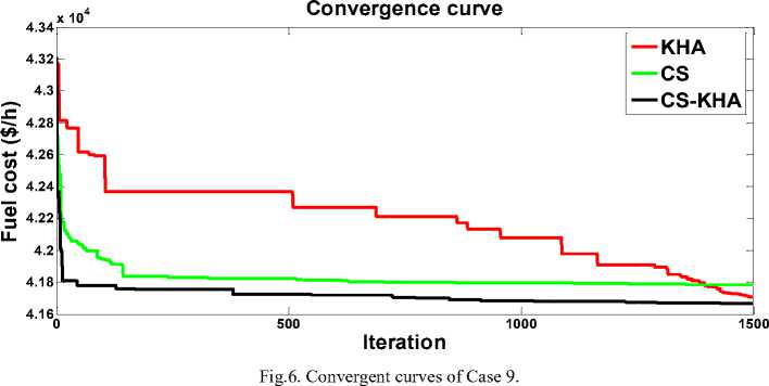
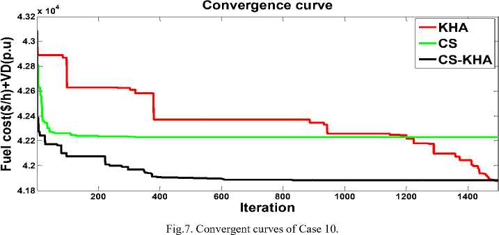
Table 10. The control variables’ optimal settings for case11.

Control variable CS-KHA		KHA  CS		Control variable      CS-KHA			KHA CS
P G1 (MW)	366.9132	385.4828	368.0476	V G1 (p.u)	1.0322	1.0169	1.0043
P G4 (MW)	30.0000	30.0000	40.4392	V G4 (p.u)	1.0515	1.0342	1.0224
P G6 (MW)	30.8504	30.0000	30.0056	V G6 (p.u)	1.0349	1.0323	1.0137
P G8 (MW)	30.0000	36.5892	30.5938	V G8 (p.u)	1.0742	1.0906	1.0714
P G10 (MW)	32.1926	30.0951	30.6092	V G10 (p.u)	1.0786	1.0965	1.0833
P G12 (MW)	322.0172	337.7073	298.7903	V G12 (p.u)	1.0353	1.0238	1.0114
P G15 (MW)	66.9864	67.3679	73.6602	V G15 (p.u)	1.0383	1.0268	1.0176
P G18 (MW)	34.9502	31.6466	34.1581	V G18 (p.u)	1.0476	1.0328	1.0167
P G19 (MW)	30.0126	30.1197	34.9399	V G19 (p.u)	1.0464	1.0356	1.0192
P G24 (MW)	31.2758	40.0241	32.0601	V G24 (p.u)	1.0571	1.0634	1.0366
P G25 (MW)	30.0890	30.3142	30.7494	V G25 (p.u)	1.0939	1.0568	1.0337
P G26 (MW)	152.1116	160.5087	124.9473	V G26 (p.u)	1.0835	1.0689	1.0860
P G27 (MW)	210.4531	212.1246	213.9664	V G27 (p.u)	1.0684	1.0325	1.0148
P G31 (MW)	30.0107	30.0000	32.9586	V G31 (p.u)	1.0559	1.0328	1.0147
P G32 (MW)	32.1135	32.1022	32.1000	V G32 (p.u)	1.0628	1.0410	1.0174
P G34 (MW)	30.1433	30.0000	30.0574	V G34 (p.u)	1.0699	1.0429	1.0476
P G36 (MW)	30.9994	32.3755	37.3000	V G36 (p.u)	1.0709	1.0615	1.0452
P G40 (MW)	37.2945	31.1420	39.2771	V G40 (p.u)	1.0584	1.0335	1.0348
P G42 (MW)	32.7803	40.1303	32.0453	V G42 (p.u)	1.0728	1.0407	1.0430
P G46 (MW)	30.5901	30.0504	61.3421	V G46 (p.u)	1.0779	1.0699	1.0825
P G49 (MW)	35.7090	35.7110	35.7293	V G49 (p.u)	1.0838	1.0856	1.0880
P G54 (MW)	150.1344	159.3915	147.9769	V G54 (p.u)	1.0743	1.0686	1.0785
P G55 (MW)	45.0829	45.1069	46.4248	V G55 (p.u)	1.0661	1.0609	1.0791
P G56 (MW)	30.2316	30.1951	30.0706	V G56 (p.u)	1.0747	1.0669	1.0783
P G59 (MW)	41.1021	34.2682	31.4284	V G59 (p.u)	1.0929	1.0880	1.0949
P G61 (MW)	128.9333	126.3616	116.7174	V G61 (p.u)	1.0857	1.0959	1.0989
P G62 (MW)	119.4878	104.4463	108.5139	V G62 (p.u)	1.0857	1.0980	1.0949
P G65 (MW)	30.0414	30.6740	33.8130	V G65 (p.u)	1.0886	1.0891	1.0524
P G66 (MW)	274.4206	296.6764	274.6836	V G66 (p.u)	1.0981	1.1000	1.0983
P G69 (MW)	290.2244	273.8381	285.3788	V G69 (p.u)	1.0819	1.0947	1.0921
P G70 (MW)	33.8793	31.0321	30.0310	V G70 (p.u)	1.0760	1.0680	1.0753

P G72 (MW)	30.0000	30.0000	30.5010	V G72 (p.u)	1.0847	1.0782	1.0618
P G73 (MW)	35.0183	30.0011	34.5178	V G73 (p.u)	1.0807	1.0823	1.0806
P G74 (MW)	30.0000	34.6584	30.0089	V G74 (p.u)	1.0614	1.0721	1.0635
P G76 (MW)	31.1843	30.0000	30.0515	V G76 (p.u)	1.0481	1.0534	1.0537
P G77 (MW)	30.8112	30.0330	35.3680	V G77 (p.u)	1.0530	1.0533	1.0694
P G80 (MW)	353.3451	328.0506	339.0098	V G80 (p.u)	1.0578	1.0871	1.0748
P G85 (MW)	30.4117	34.3764	30.0251	V G85 (p.u)	1.0698	1.0849	1.0867
P G87 (MW)	31.2043	31.2010	31.2000	V G87 (p.u)	1.0883	1.0856	1.0802
P G89 (MW)	373.0515	343.3753	383.0308	V G89 (p.u)	1.0766	1.1000	1.0966
P G90 (MW)	30.0217	30.0053	30.0816	V G90 (p.u)	1.0543	1.0908	1.0790
P G91 (MW)	30.1360	31.2499	33.4771	V G91 (p.u)	1.0621	1.0926	1.0810
P G92 (MW)	30.0000	31.6228	30.0239	V G92 (p.u)	1.0568	1.0932	1.0839
P G99 (MW)	31.5839	30.1290	32.1729	V G99 (p.u)	1.0515	1.0699	1.0605
P G100 (MW)	161.0126	174.5208	163.4482	V G100 (p.u)	1.0395	1.0786	1.0654
P G103 (MW)	42.2950	42.1514	42.2731	V G103 (p.u)	1.0212	1.0726	1.0593
P G104 (MW)	30.8340	31.1019	30.1950	V G104 (p.u)	1.0060	1.0641	1.0498
P G105 (MW)	30.1658	30.0082	30.0294	VG105 (p.u)	1.0123	1.0751	1.0472
P G107 (MW)	30.7389	30.1938	30.7178	V G107 (p.u)	0.9973	1.0717	1.0433
P G110 (MW)	32.0056	30.6153	30.4068	V G110 (p.u)	0.9894	1.0791	1.0417
P G111 (MW)	40.8006	40.8581	40.8015	V G111 (p.u)	0.9980	1.0890	1.0528
P G112 (MW)	30.6941	30.1776	35.3112	V G112 (p.u)	0.9775	1.0721	1.0298
P G113 (MW)	30.5556	30.1612	43.2123	V G113 (p.u)	1.0584	1.0584	1.0260
P G116 (MW)	31.5470	30.1511	30.6720	V G116 (p.u)	1.0928	1.1000	1.0466
Qc 5 (Mvar)	1.0968	0.1341	0.4603	T (8–5)         1.0269   1.0527  1.0180
Qc 34 (Mvar)	0.0395	0.0656	7.8806	T (26–25)	1.0551	0.9293	1.0770
Qc 37 (Mvar)	1.7660	7.3596	2.7258	T (30–17)	0.9923	1.0165	1.0267
Qc 44 (Mvar)	10.4951	0.3568	0.0083	T (38–37)	0.9561	0.9903	0.9672
Qc 45 (Mvar)	0.0001	2.6926	1.0940	T (63–59)	0.9402	0.9071	0.9072
Qc 46 (Mvar)	6.3599	0.6672	17.7909	T (64–61)	1.0339	0.9722	0.9434
Qc 48 (Mvar)	0.3103	0.6422	0.3959	T (65–66)	1.0317	1.0952	1.0250
Qc 74 (Mvar)	0.5937	0.0949	12.9769	T (68–69)	1.0046	1.0947	0.9504
Qc 79 (Mvar)	0.4359	1.0046	1.7815	T (81–80)	1.0284	0.9213	0.9667
Qc 82 (Mvar)	2.6580	0	2.5440
Qc83(Mvar)	2.7523	0	2.0127	Objective functions
Qc 105 (Mvar)	1.1846	2.5892	10.9604	Fuel cost ($/h) 135260.45		135400.78	135610.321
Qc 107 (Mvar)	4.1717	0.0284	4.9321	Ploss (MW)   56.4548  58.1287			53.3527
Qc 110 (Mvar)	4.0167	0.57250.0614

Table 11. The results obtained are compared for Case 11.

Case	Algorithms	Fuel cost ($/h)
	CS-KHA	135260.45
Case 11	KHA	135400.78
	CS	135610.321
	BSA [37]	135333.4743
	ABC [37]	135304.3584
	BBO [37]	135263.7289

• [1]    Shaheen, A.M., El-Sehiemy, R.A., Farrag, S.M., "Solving multi-objective optimal power flow problem via forced initialised differential evolution algorithm," IET Generation, Transmission and Distribution 2016, 10(7), pp. 1634-1647

• [2]    Huneault M, Galiana FD. A survey of the optimal power flow literature. IEEE Trans Power Syst 1991; 6(2):762–70.

• [3]    Chowdhury B, Rahman S. A review of recent advances in economic dispatch. IEEE Trans Power Syst 1990; 5 (4): 1248–59.

• [4]    T. Niknam, M. Rasoul Narimani, M. Jabbari, A.R. Malekpour, A modified shuffle frog leaping algorithm for multi-objective optimal power flow, Energy 36 (2011) 6420–6432,

• [5]    Roa-Sepulveda C, Pavez-Lazo B. A solution to the optimal power flow using simulated annealing. Int J Electri Power Energy Syst 2003; 25:47–57.

• [6]    L.L. Lai & J.T. Ma. Improved genetic algorithms for optimal power flow under both normal and contingent

  operation states. Electrical Power and Energy Systems, 19, 287-292, 1997.

• [7]    S.R. Paranjothi, K. Anburaja, Optimal power flow using refined genetic algorithm, Electr. Power Components Syst. 30 (2002) 1055–1063.

• [8]    Shaheen, A.M., Farrag, S.M., El-Sehiemy, R.A., "MOPF solution methodology,", IET Generation, Transmission and Distribution 2017 11(2), pp. 570-581

• [9]    M. Abido, Optimal power flow using Tabu search algorithm, Electric Power Syst. Res. 30 (2002) 469–483.

• [10]    Ghasemi M, Ghavidel S, Ghanbarian MM, Massrur HR, Gharibzadeh M. Application of imperialist competitive algorithm with its modified techniques for multi-objective optimal power flow problem: a comparative study. Inf Sci (Ny) 2014; 281:225–47.

• [11]    M. A. Abido, Optimal power flow using particle swarm optimization, Electrical Power and Energy Systems, 24, 563-571, 2002.

• [12]    A. Ramesh Kumar & L. Premalatha, Optimal power flow for a deregulated power system using adaptive real coded biogeography-based optimization, Electrical Power and Energy Systems, 73,393–399, 2015.

• [13]    P.K. Roy, S.P. Ghoshal, S.S. Thakur, Biogeography based optimization for multi-constraint optimal power flow with emission and non-smooth cost function, Expert Syst. Appl. 37 (2010) 8221–8228.

• [14]    Bhattacharya, A.,  & Chattopadhyay, P. K. (2011).

• [15]    El-Sehiemy, R.A., Shafiq, M.B., Azmy, A.M., "Multiphase search optimization algorithm for constrained optimal power flow problem," International Journal of Bio-Inspired Computation, 2014, 6(4), pp. 275-289.

• [16]    R. Roy & H.T. Jadhav, Optimal power flow solution of power system incorporating stochastic wind power using Gbest guided artificial bee colony algorithm, Electrical Power and Energy Systems, 64, 562–578, 2015.

• [17]    A.R. Bhowmik, A.K. Chakraborty, Solution of optimal power flow using non dominated sorting multi objective opposition based gravitational search algorithm, Int. J. Electr. Power Energy Syst. 64 (2015) 1237–1250.

• [18]    K. Ayan, U. Kılıc¸, B. Baraklı, Chaotic artificial bee colony algorithm based solution of security and transient stability constrained optimal power flow, Int. J. Electr. Power Energy Syst. 64 (2015) 136–147.

• [19]    L. Dilip, R. Bhesdadiya, P. Jangir, Optimal Power Flow Problem Solution Using Multi-objective Grey Wolf Optimizer Algorithm, Springer Nature Singapore, Pte. Ltd. 2018.

• [20]    Bouchekara HREH. Optimal power flow using blackhole-based optimization approach. Appl Soft Comput J 2014; 24:879–88.

• [21]    Bouchekara HREH, Abido Ma, Boucherma M. Optimal power flow using teaching-learning-based optimization technique. Electr Power Syst Res 2014; 114:49–59.

• [22]    Attia, A.-F., El Sehiemy, R.A., Hasanien, H.M., "Optimal power flow solution in power systems using a novel SineCosine algorithm," International Journal of Electrical Power and Energy Systems, 2018, 99, pp. 331-343

• [23]    Daryani N, Hagh MT, Teimourzadeh S. Adaptive group search optimization algorithm for multi-objective optimal power flow problem. Appl Soft Comput 2016; 38:1012– 24.

• [24]    A. Khelifi, S. Chettih, B. Bentouati, A new hybrid algorithm of particle swarm optimizer with grey wolves’ optimizer for solving optimal power flow problem, Leonardo Electronic J. of P. & Technologies. 2018, 249270.

• [25]    M. AlRashidi, M. El-Hawary, Applications of computational intelligence techniques for solving the revived optimal power flow problem, Electr. Power Syst. Res. 79 (2009) 694–702.

• [26]    A.H. Gandomi, A.H. Alavi, Krill herd: a new bio-inspired optimization algorithm, Commun. Nonlinear Sci. Numer. Simulat. 17 (2012) 4831–4845.

• [27]    Wang G-G, Guo L, Gandomi AH, Hao G-S, Wang H, Chaotic krill herd algorithm. Inf Sci 274 (2014) 17-34.

• [28]    Bentouati, B., Chettih, S., El-Sehiemy, R., "A chaotic firefly algorithm framework for non-convex economic dispatch problem," Electrotehnica, Electronica, Automatica (EEA), 2018, 66(1), pp. 172-179

• [29]    Xin-She Yang, Flower Pollination Algorithm for Global Optimization. In: Unconventional Computation and Natural Computation, Vol. 7445, Springer Lecture Notes in Computer Science, Berlin, Heidelberg, 2012, pp. 240– 249.

• [30]    Ghasemia M, Taghizadeh M, Ghavidel S, Abbasian A. Colonial competitive differential evolution:   an

  experimental study for optimal economic load dispatch. Appl Soft Comput 2016; 40:342e63.

• [31]    B. Mandal, P. Kumar Roy, Multi-objective optimal power flow using quasi-oppositional teaching–learning-based optimization, Appl. Soft Comput. 21(2014) 590–606.

• [32]    Bouchekara, H. R. E. H., Chaib, A. E., Abido, M. A., & El-Sehiemy, R. A. (2016). Optimal power flow using an Improved Colliding Bodies Optimization algorithm. Applied Soft Computing, 42, 119-131.

• [33]    Mohamed, A. A. A., Mohamed, Y. S., El-Gaafary, A. A., & Hemeida, A. M. (2017). Optimal power flow using moth swarm algorithm. Electric Power Systems Research, 142, 190-206.

• [34]    Bachir Bentouati et al, Optimal Power Flow using the Moth Flam Optimizer: A case study of the Algerian power system, TELKOMINIKA,.1, pp. 3. 2016.

• [35]    Bentouati, B., Chettih, S., El Sehiemy, R., Wang, G.-G. , "Elephant herding optimization for solving non-convex optimal power flow problem," Journal of Electrical and Electronics Engineering, 201710(1), pp. 31-36

• [36]    Bentouati, B., Chettih, S., Djekidel, R., El-Sehiemy, R.A., "An efficient chaotic cuckoo search framework for solving non-convex optimal power flow problem," International Journal of Engineering Research in Africa, 2017, 33, pp. 84-99

• [37]    Chaib, A. E., Bouchekara, H. R. E. H., Mehasni, R., & Abido, M. A. (2016). Optimal power flow with emission and non - smooth cost functions using backtracking search optimization algorithm. International Journal of Electrical Power & Energy Systems, 81, 64-77.

• [38]    Wang G, Gandomi AH, Alavi AH. An effective krill herd algorithm with migration operator in biogeography-based optimization. Appl Math Model 2014; 38(9-10):2454–62.

• [39]    El-Hosseini, M.A., El-Sehiemy, R.A., Haikal, A.Y.,

"Multi-objective optimization  algorithm  for secure economical/emission dispatch problems,"  Journal of

Engineering and Applied Science, 2014 61(1), pp. 83-103

• [40]    Biswas, P. P., Suganthan, P. N., & Amaratunga, G. A. (2017). Optimal power flow solutions incorporating stochastic wind and solar power. Energy Conversion and Management, 148, 1194-1207.

• [41]    H. R. E. H. Bouchekara, Chaib, A. E., & Abido, M. A. Optimal power flow using GA with a new multi-parent crossover considering: prohibited zones, valve-point effect, multi-fuels and emission. Electr Eng (2016).

• [42]    Kessel, P., & Glavitsch, H. (1986). Estimating the voltage stability of a power system. IEEE Transactions on Power Delivery, 1(3), 346-354.

• [43]    R.D. Zimmerman, C.E. Murillo-Sánchez, R.J. Thomas, Matpower (Available at :) http:// www. pserc. cornell. edu/ matpower.