A Novel Hybrid PSO-GSA Method for Non-convex Economic Dispatch Problems

Published Online November 2013 in MECS DOI: 10.5815/ijieeb.2013.05.01

The economic dispatch (ED) problem is one of the fundamental issues in power system operation and control. The ED problem finds the optimum allocation of load among the committed generating units subject to satisfaction of power balance and capacity constraints, such that the total cost of operation is kept at a minimum. Various methods and investigations are being carried out until date in order to produce a significant saving in the operational cost. Traditionally, fuel cost function of a generator is represented by single quadratic function. But a quadratic function is not able to show the practical behavior of generator. For modeling of the practical cost function behavior of a generator, a non-convex curve is used in literature. The ED problem is a non-convex and nonlinear optimization problem. Due to ED complex and nonlinear characteristics, it is hard to solve the problem using classical optimization methods.

Most of classical optimization techniques such as lambda iteration method, gradient method, Newton’s method, linear programming, Interior point method and dynamic programming have been used to solve the basic economic dispatch problem [1]. These mathematical methods require incremental or marginal fuel cost curves which should be monotonically increasing to find global optimal solution. In reality, however, the input-output characteristics of generating units are non-convex due to valve-point loadings and multi-fuel effects, etc. Also there are various practical limitations in operation and control such as ramp rate limits and prohibited operating zones, etc. Therefore, the practical ED problem is represented as a non-convex optimization problem with equality and inequality constraints, which cannot be solved by the traditional mathematical methods. Dynamic programming (DP) method [2] can solve such types of problems, but it suffers from so-called the curse of dimensionality. Over the past few decades, as an alternative to the conventional mathematical approaches, many salient methods have been developed for ED problem such as genetic algorithm (GA) [3], improved tabu search (TS) [4], simulated annealing (SA) [5], neural network (NN) [6], evolutionary programming (EP) [7]-[9], biogeography-based optimization (BBO) [10], particle swarm optimization (PSO) [13]-[16], differential evolution (DE) [17], and gravitational search algorithm (GSA) [18].

PSO is a stochastic algorithm that can be applied to nonlinear optimization problems. PSO has been developed from the simulation of simplified social systems such as bird flocking and fish schooling by Kennedy and Eberhart [11], [12]. The main difficulty classic PSO is its sensitivity to the choice of parameters and they also premature convergence, which might occur when the particle and group best solutions are trapped into local minimums during the search process. One of the recently improved heuristic algorithms is the gravitational search algorithm (GSA) based on the Newton’s law of gravity and mass interactions. GSA has been verified high quality performance in solving different optimization problems in the literature [19]. The same goal for them is to find the best outcome (global optimum) among all possible inputs. In order to do this, a heuristic algorithm should be equipped with two major characteristics to ensure finding global optimum. These two main characteristics are exploration and exploitation [20].

In this paper, a novel and efficient approach is proposed to solve the non-convex ED problems using a new hybrid PSO-GSA technique. The performance of the proposed approach has been demonstrated on two different test systems, i.e. 6-unit and 13-unit systems. Obtained simulation results demonstrate that the proposed method provides very remarkable results for solving the ED problem. The results have been compared to those reported in the literature.

• II.    PROBLEM FORMULATION

• 2.1    ED Problem

The objective of an ED problem is to find the optimal combination of power generations that minimizes the total generation cost while satisfying equality and inequality constraints. The fuel cost curve for any unit is assumed to be approximated by segments of quadratic functions of the active power output of the generator. For a given power system network, the problem may be described as optimization (minimization) of total fuel cost as defined by (1) under a set of operating constraints.

nn

F t = E F i ( P ) = E ( a . P ² + bP + d (1) i = 1                      i = 1

where F_T is total fuel cost of generation in the system ($/hr), a i , b i , and c i are the cost coefficient of the i -th generator, P_i is the power generated by the i -th unit and n is the number of generators.

• (i)    Active Power Balance Equation

For power balance, an equality constraint should be satisfied. The total generated power should be the same as total load demand plus the total line loss.

n

E P . = P d + P oss                        (2)

i = 1

where PD is the total load demand and PLoss is total transmission losses. The transmission losses PLoss can be calculated by using B matrix technique and is defined by (3) as, nn        n

Loss                  i ij j             0 i i 00

i = 1 j = 1                     i = 1

where B ij is coefficient of transmission losses and the B_0i and B₀₀ is matrix for loss in transmission which are constant under certain assumed conditions.

• (ii)    Minimum and Maximum Power Limits

Generation output of each generator should lie between minimum and maximum limits. The corresponding inequality constraint for each generator is

P ^min <  P <  P ^ma x for i = 1,2, ■ ■ , n             (4)

where P_i ^min and P_i ^max are the minimum and maximum outputs of the i- th generator, respectively.

• (iii)    Ramp Rate Limits

The actual operating ranges of all on-line units are restricted by their corresponding ramp rate limits. The ramp-up and ramp-down constraints can be written as (5) and (6), respectively.

P ( t ) - P ( t - 1) <  UR.                        (5)

P ( t - 1) - P ( t ) <  dr .

where P ( t ) and P ( t -1) are the present and previous power outputs, respectively. UR and DR are the rampup and ramp-down limits of the - th generator.

To consider the ramp rate limits and power output limits constraints at the same time, therefore, eqs. (4), (5) and (6) can be rewritten as follows:

max{ P ^mn, P ( t - 1) - DR . } <  P ( t ) <  min{ P ^max, P ( t - 1) + UR . }

• ( v) Proh b ted Operat ng Zones

The generating units with prohibited operating zones have discontinuous and nonlinear cost characteristics. This characteristic can be formulated in ED problems as follows:

^P i ^‘

min P

u

P i' , k - 1

< P - <  P J

< P <  P*_k , k = 2,3, ^ , pz.       (8)

u              max

• ¹    i , pz —¹i—¹i , ¹ b^,***, n pz

• 2.2 ED Problem w th Valve Po nt Effect

where P _, ^l _k and P _, ^u _k are the lower and upper boundary of prohibited operating zone of unit , respectively. Here, pz is the number of prohibited zones of unit and n_pz is the number of units which have prohibited operating zones.

For more rational and precise modeling of fuel cost function, the above expression of cost function is to be modified suitably. The generating units with multivalve steam turbines exhibit a greater variation in the fuel-cost functions [14]. The valve opening process of multi-valve steam turbines produces a ripple-like effect in the heat rate curve of the generators . These “valvepoint effects” are illustrated in Fig. 1.

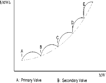
C : Tertiary Valve D : Quaternary Valve

E : Quinary Valve

k + 1       k

X i   = X i

w = w

max

, £+1

⁺ v

(wrnax---wrnin, l   Itermax   )

x Iter

Figure . 1: Valve-point effect

The significance of this effect is that the actual cost curve function of a large steam plant is not continuous but more important it is non-linear. The valve-point effects are taken into consideration in the ED problem by superimposing the basic quadratic fuel-cost characteristics with the rectified sinusoid component as follows:

where v ^t is velocity of particle at iteration t, w is inertia factor, c 1 and c 2 are accelerating factor, r 1 and r 2 are positive random number between 0 and 1, pbest is the best position of particle , gbest is the best position of the group, w_max and w_{m n} are maximum and minimum of inertia factor, Iter_max is maximum iteration, n is number of particles.

Fig. 2 shows the concept of the searching mechanism of PSO using the modified velocity and position of individual based on (10), (11) and (12) if the value of w , c 1 , c 2 , r 1 , and r 2 are 1.

n

F t = Z F ( P )

i = 1

i = 1

' a P i ² + b i P i + c i +

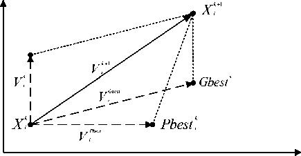
Figure . 2: Concept of modification of searching point by PSO

e i x sin ( f i x ( P i ^min

—

where F T is total fuel cost of generation in ($/hr) including valve point loading, e i , f i are fuel cost coefficients of the i- th generating unit reflecting valvepoint effects.

• III.    META-HEURISTIC OPTIMIZATION

  • 3.1    Overview of Particle Swarm Optimization

The particle swarm optimization (PSO) algorithm is introduced by Kennedy and Eberhart based on the social behavior metaphor. In PSO a potential solution for a problem is considered as a bird without quality and volume, which is called a particle, flying through a D-dimensional space, adjusting its position in search space according to its own experience and its neighbors. In PSO, the i- th particle is represented by its position vector x_i in the D-dimensional space and its velocity vector v_i . In each time step t , the particles calculate their new velocity then update their position according to equations (10) and (11) respectively.

Vt+1 = w x vi + c1 x r x (pb c2 x r2 x (gbest — x\ xt ) +

i

)

The process of implementing the PSO is as follows:

Step 1: Create an initial population of individual with random positions and velocity within the solution space.

Step 2: For each individual, calculate the value of the fitness function.

Step 3: Compare the fitness of each individual with each Pbest . If the current solution is better than its Pbest , then replace its Pbest by the current solution.

Step 4: Compare the fitness of all individual with Gbes t. If the fitness of any individual is better than Gbest , then replace Gbest .

Step 5: Update the velocity and position of all individual according to (10) and (11).

Step 6: Repeat steps 2-5 until a criterion is met.

• 3.2    Grav tat onal Search Algor thm (GSA)

Rashedi et al. proposed one of the newest heuristic algorithms, namely Gravitational Search Algorithm (GSA) in 2009. GSA is based on the physical law of gravity and the law of motion. The gravitational force between two particles is directly proportional to the product of their masses and inversely proportional to the square of the distance between them [19]. GSA a set of agents called masses has been proposed to find the optimum solution by simulation of Newtonian laws of gravity and motion. In the GSA, consider a system with m masses in which position of the i-th mass is defined as follows:

X, =( x1,_, xd..... xn), i = 1,2,..., m

where x_i^d is position of the i-th mass in the d-th dimension and n is dimension of the search space. At the specific time t a gravitational force from mass j acts on mass i , and is defined as follows:

G ( t ) = G ( G o , t )

G ( t ) = G о e T

The masses of the agents are calculated using fitness evaluation. A heavier mass means a more efficient agent. This means that better agents have higher attractions and moves more slowly. Supposing the equality of the gravitational and inertia mass, the values of masses is calculated using the map of fitness. The gravitational and inertial masses are updating by the following equations:

F j ( t ) = G ( t )

M p. (t ) -' M j (t ) R y ⁽ t) + £

m ( t ) = /zt X t ) - worst ⁽ t )

¹      best ( t ) - worst ( t )

[( x j ( t ) - x d ( t ) )

where M is the mass of the object , M j is the mass of the object j , G(t) is the gravitational constant at time t , R j (t) is the Euclidian distance between the two objects and j , and ε is a small constant.

The total force acting on agent in the dimension d is calculated as follows:

m ( t )

М ( t ) = m

У ^ m y ⁽ t ) ^j = 1                                                (22)

m

F d ( t ) = £ rand y F j ( t )

y = 1

j * i

where f t (t) represents the fitness value of the agent at time t , and the best(t) and worst(t) in the population respectively indicate the strongest and the weakest agent according to their fitness route. For a minimization problem:

best ( t ) = min ft j ( t ) j e [ 1, ^ , m ]     ^J

where rand j is a random number in the interval [0, 1].

According to the law of motion, the acceleration of the agent , at time t , in the d-th dimension, a ^d ( t ) is given as follows:

worst ( t ) = max ft j ( t ) j e [ 1, _ , m ] ^J

a . ( t) =

F ^d ( t )

M ( t )

Furthermore, the next velocity of an agent is a function of its current velocity added to its current acceleration. Therefore, the next position and the next velocity of an agent can be calculated as follows:

v d ( t + 1) = rand x v d ( t ) + a^d ( t )

x d ( t + 1) = x d ( t ) + v d (t + 1)

where rand is a uniform random variable in the interval [0, 1].

The gravitational constant, G , is initialized at the beginning and will be decreased with time to control the search accuracy. In other words, G is a function of the initial value ( G 0 ) and time t :

The GSA approach for optimization problem can be summarized as follows [19]:

Step 1: Search space identification,

Step 2: Generate initial population between minimum and maximum values,

Step 3: Fitness evaluation of agents,

Step 4: Update G(t), best(t), worst(t) and M (t) for = 1,2,. . .,m ,

Step 5: Calculation of the total force in different directions,

Step 6: Calculation of acceleration and velocity,

Step 7: Updating agents’ position,

Step 8: Repeat step 3 to step 7 until the stop criteria is reached,

Step 9: Stop.

3.3 The Hybr d PSO-GSA

A hybrid PSO-GSA approach is an integrated approach between PSO and GSA which combines the ability of social thinking ( gbest ) in PSO with the local search capability of GSA. In order to combine these

algorithms, the updated velocity of agent i can be calculated as follows:

V i ( t + 1) = w x V i ( t ) + c 1 x rand, x a i ( t ) + c 2 x rand, x ( gbest - X . ( t ) )

where V i (t) is the velocity of agent i at iteration t , c j is a weighting factor, w is a weighting function, rand is a random number between 0 and 1, a_i (t) is the acceleration of agent i at iteration t , and gbest is the best solution so far.

The position of the particles at each iteration updated as follow:

X ( t + 1) = x, ( t ) + V ( t )

The process of the proposed PSO-GSA algorithm can be summarized as the following steps:

Step 1: Get the data for the system,

Step 2: Generate initial population,

Step 3: Fitness evaluation of agents,

Step 4: Update G(t) and gbest(t) ,

Step 5: Calculation of the mass of the object, gravitational constant, the total force, and acceleration,

Step 6: Updating agents’ velocity and position,

Step 7: Repeat step 3 to step 6 until the stop criteria is reached,

Step 8: Stop.

• IV.    SIMULATION RESULTS

To verify the feasibility of the proposed technique, two different power systems were tested: (1) 6-unit system considering power loss, ramp rate limits and prohibited operating zones; and (2) 13-unit system with valve-point effects and transmission losses are neglected.

Test Case 1: 6-unit system

The system consists of six thermal generating units. The total load demand on the system is 1263 MW. The parameters of all thermal units are presented in Table 1 and Table 2 [13], followed by the transmission loss B matrices.

The obtained results for the 6-unit system using the hybrid PSO-GSA method are given in Table 3 and the results are compared with other methods reported in literature, including GA, PSO and IDP [21], RGA and GA-PSO [22]. It can be observed that PSO-GSA can get total generation cost of 15,441 ($/hr) and power losses of 12.2417 (MW), which is the best solution among all the methods. Note that the outputs of the generators are all within the generator’s permissible output limit.

TABLE 1: Cost coefficients and unit operating limits

Unit	P min (MW)	P max (MW)	a	b	c
1	100	500	0.0070	7.0	240
2	50	200	0.0095	10.0	200
3	80	300	0.0090	8.5	220
4	50	150	0.0090	11.0	200
5	50	200	0.0080	10.5	220
6	50	120	0.0075	12.0	190

TABLE 2: Ramp rate limits and prohibited operating zones

Unit	P 0 (MW)	UR i (MW/h)	DR i (MW/h)	Prohibited zones (MW)
1	440	80	120	[210, 240] [350, 380]
2	170	50	90	[90, 110] [140, 160]
3	200	65	100	[150, 170] [210, 240]
4	150	50	90	[80, 90] [110, 120]
5	190	50	90	[90, 110] [140, 150]
6	110	50	90	[75, 85] [100, 105]

	0.0017  0 . 0012  0.0007 - 0.0001 - 0.0005 - 0.0002 0.0012  0 . 0014  0.0009  0.0001 -0.0006 -0.0001 0.0007  0 . 0009  0.0031  0.0000 -0.0010 -0.0006
B j =	- 0.0001 0 . 0001 0.0000 0.0024 -0.0006 - 0.0008 - 0.0005 -0 . 0006 -0.0010 -0.0006 0.0129 -0.0002 - 0.0002 -0 . 0001 -0.0006 -0.0008 -0.0002  0.0150

B 0 i = 1.0 e ^: *[ - 0.3908 - 0.1297 0.7047 0.0591 0.2161 - 0.6635 ]

B ₀₀ = 0.0056

Test Case 2: 13-unit system

The second system consists of 13 generating units and the input data of 13-generator system are given in Table 4 [8]. In this sample system consisting of thirteen generators with valve-point loading effects and have a total load demands of 1800 MW and 2520 MW, respectively.

The best fuel cost result obtained from proposed method and other optimization algorithms are compared in Table 5 and Table 6 for load demands of 1800 MW and 2520 MW, respectively. In Table 5, generation outputs and corresponding cost obtained by the proposed method are compared with those of NN-EPSO, EP-EPSO, and GSA [18, 23]. The proposed algorithm provides a better solution (total generation cost of 17909.2396 $/hr) than other methods while satisfying the system constraints.

TABLE 3: Comparison of the best results of each methods (P D = 1263 MW)

Unit Output	GA	PSO	IDP	RGA	GA-PSO	PSO-GSA
P1 (MW)	474.8066	447.4970	450.9555	420.2342	431.5408	446.6525
P2 (MW)	178.6363	173.3221	173.0184	199.4412	184.272	172.8814
P3 (MW)	262.2089	263.0594	263.6370	263.7234	259.7322	262.5411
P4 (MW)	134.2826	139.0594	138.0655	120.0030	138.8306	143.1982
P5 (MW)	151.9039	165.4761	164.9937	167.2319	168.6130	163.6354
P6 (MW)	74.1812	87.1280	85.3094	105.1250	92.4211	86.3387
Total power output (MW)	1276.0217	1275.9584	1275.9794	1275.7588	1275.4093	1275.2417
Total generation cost ($/hr)	15,459	15,450	15,450	15,461.3	15,446.1	15,441
Power losses (MW)	13.0217	12.9584	12.9794	12.7588	12.4093	12.2417

TABLE 4: Generating units capacity and coefficients (13-units)

Unit	P min (MW)	P max (MW)	a	b	c	e	f
1	0	680	0.00028	8.10	550	300	0.035
2	0	360	0.00056	8.10	309	200	0.042
3	0	360	0.00056	8.10	307	200	0.042
4	60	180	0.00324	7.74	240	150	0.063
5	60	180	0.00324	7.74	240	150	0.063
6	60	180	0.00324	7.74	240	150	0.063
7	60	180	0.00324	7.74	240	150	0.063
8	60	180	0.00324	7.74	240	150	0.063
9	60	180	0.00324	7.74	240	150	0.063
10	40	120	0.00284	8.60	126	100	0.084
11	40	120	0.00284	8.60	126	100	0.084
12	55	120	0.00284	8.60	126	100	0.084
13	55	120	0.00284	8.60	126	100	0.084

TABLE 5: Comparison of the best results of each methods (P D = 1800 MW)

Unit power output	NN-EPSO [23]	EP-EPSO [23]	GSA [18]	PSO-GSA
P1 (MW)	490.0000	505.4731	628.3185	552.9874
P2 (MW)	189.0000	254.1686	149.5996	261.6571
P3 (MW)	214.0000	253.8022	222.7492	261.5613
P4 (MW)	160.0000	99.8350	109.8666	100.7864
P5 (MW)	90.0000	99.3296	109.8665	100.7889
P6 (MW)	120.0000	99.3035	109.8665	60.0000
P7 (MW)	103.0000	99.7772	109.8665	100.7048
P8 (MW)	88.0000	99.0317	60.0000	100.7799
P9 (MW)	104.0000	99.2788	109.8666	100.7342
P10 (MW)	13.0000	40.0000	40.0000	40.0000
P11 (MW)	58.0000	40.0000	40.0000	40.0000
P12 (MW)	66.0000	55.0000	55.0000	55.0000
P13 (MW)	55.0000	55.0000	55.0000	55.0000
Total power output (MW)	1800	1800	1800	1800
Total generation cost ($/h)	18442.5931	17932.4766	17960.3684	17909.2396

TABLE 6: Comparison of the best results of each methods (P D = 2520 MW)

Unit power output	GA-SA [23]	PSO-SQP [23]	GSA [18]	PSO-GSA
P1 (MW)	628.23	628.3205	628.3185	679.8605
P2 (MW)	299.22	299.0524	299.1993	359.9998
P3 (MW)	299.17	298.9681	294.5730	360.0000
P4 (MW)	159.12	159.4680	159.7331	154.3514
P5 (MW)	159.95	159.1429	159.7331	158.1922
P6 (MW)	158.85	159.2724	159.7331	149.0500
P7 (MW)	157.26	159.5371	159.5371	156.2124
P8 (MW)	159.93	158.8522	159.7331	151.6807
P9 (MW)	159.86	159.7845	159.7331	159.3809
P10 (MW)	110.78	110.9618	77.3999	40.0972
P11 (MW)	75.00	75.0000	77.3999	41.0277
P12 (MW)	60.00	60.0000	92.3999	55.1472
P13 (MW)	92.62	91.6401	92.3999	55.0000
Total power output (MW)	2520	2520	2520	2520
Total generation cost ($/h)	24275.71	24261.05	24164.2514	24140.8005

In Table 6, generation outputs and corresponding cost obtained by the proposed method are compared with those of GA-SA, PSO-SQP, and GSA [18, 23]. The hybrid PSO-GSA provides a better solution (total generation cost of 24140.8005 $/hr) than other methods while satisfying the system constraints. We have also observed that the solutions using hybrid PSO-GSA algorithm always are satisfied with the equality and inequality constraints.

• V.    CONCLUSION

In this paper, a new hybrid PSO-GSA technique has been applied to solve the non-convex ED problem of generating units considering the valve-point effects, prohibited operation zones, ramp rate limits and transmission losses. The proposed technique has provided the global solution in the 6-unit and 13-unit test systems and the better solution than the previous studies reported in literature. Also, the equality and inequality constraints treatment methods have always provided the solutions satisfying the constraints.