A Novel Machine Learning-Based Approach for Graph Vertex Coloring: Achieving Optimal Solutions with Scalability

A graph is a set of nodes, and edges connect these nodes. These graphs find various applications in real-life scenarios such as social networking, navigation, scheduling [1], frequency assignment [2], compiler registers [3], and more [4]. A particularly intriguing application of graph theory involves the coloring problem, which seeks to assign colors to vertices while avoiding assigning the same color to connected vertices. The goal is to minimize the number of colors used. There are different approaches to solving the coloring problem, including Integer Programming, Backtracking [5], DSATUR Algorithm [6], and a greedy algorithm. The greedy algorithm aims to find optimal solutions for all vertex–coloring problems (VCP).

To tackle intractable problems, Approximation algorithms and heuristic methods are used. These methods provide solutions that are acceptable to users, even though they might not be optimal. When employing an algorithm on a graph, it may return a feasible k-coloring approach, which is checked for usability. If it doesn't meet the criteria, other algorithms are utilized to find solutions with fewer colors. Let's consider a graph G (V, E), where V is the vertex set and E represents the Edge Set.

The graph coloring is a difficult combinatorial optimization task that may involve assigning various colors to the vertices in a graph in such a way that adjacent vertices do not share the same color. Machine learning methods, including SVMs (Support Vector Machines), offer new ways to address the graph coloring problem by using data-driven strategies to improve solution quality and efficiency. SVMs can classify graph nodes by learning from features of the graph, like node degrees, adjacency relationships, and clustering coefficients. By providing training on labeled datasets of solved graphs, SVMs are capabilities to generate accurate predictions that inform heuristic approaches for optimization.

Other machine learning approaches, such as GNNs (graph neural networks), do extremely well at encoding graph structures and establishing their relationships. GNNs learn node embeddings that capture the contextual information required for developing effective coloring strategies concerning unseen graphs. These models are refined iteratively based on feedback when paired with reinforcement learning. These models have the capability of optimizing coloring solutions over time. Supervised learning can train models for predicting heuristics or color assignments with the help of existing solved examples, while meta-learning focuses on the adaptation of various graph types by including the learning process of generalizable strategies.

A naïve approach to coloring the graph would be to use a different color for each vertex, equal to the size of the set ‘V’. However, a more optimal approach involves allowing the same color for non-adjacent vertices, considering independent sets, and repeating the process throughout the graph to minimize the number of colors used. A greedy approach can also be employed, where Graph G (V, E) is divided into sub-graphs with an equal number of vertices. These sub-graphs are then colored individually and joined at the end. However, this approach may lead to color conflicts among adjacent vertices in the subgraphs, which necessitates increasing the number of colors used in the solution. Additionally, hybrid methods may combine machine learning with optimization techniques to balance the accuracy and scalability of existing systems.

If the graph is not split around the optimized vertex, solving the problem may consume more time and space. For example, in a graph with four vertices, we can use a maximum of 4 colors [Fig. 1]. By assigning color 1 to the center node and color 2 to the remaining nodes, we can ensure that no two adjacent vertices have the same color. Hence, the authors can say that the graphs have wide-ranging applications, and the coloring problem can be approached through different algorithms and heuristic methods. The goal is to find solutions that use the minimum number of colors to avoid assigning the same color to connected vertices.

The previous method presented a simplistic approach to tackle the vertex coloring problem, suitable for cases involving a limited number of vertices. However, this method proves impractical when dealing with larger graphs containing hundreds of nodes and thousands of edges. In this approach, colors are assigned to each vertex one by one, and then the feasibility of the coloring is checked for all nodes in the graph. This repetitive process results in a complexity of nxn for a graph with n nodes, leading to an enormously large number of computations. For instance, a graph with 200 nodes would entail approximately 1.58 * 1060 computations, making it infeasible for larger graphs containing thousands of nodes.

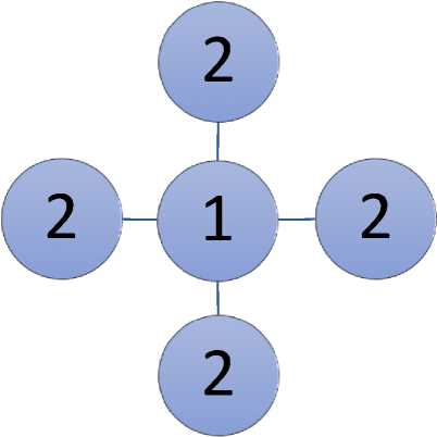
Fig. 1. Representation of a Graph with 5 nodes and 4 edges for coloring purpose.

The contributions of this paper are described below:

• i.    The authors provide mathematical theorems and proofs to achieve optimal solutions with scalability for machine learning-based approaches to graph vertex coloring.

• ii.    The authors manifested the use of Support Vector Machines to predict the best-suited algorithm for the Instances as mentioned in the (DIMACS).

• iii.    The authors constructed the hyper-plane margins by rapidly changing the time and percentage gap values from optimal solutions in correspondence to the algorithmic combination.

• iv.    The authors computed the accuracy of the proposed model, which is for any new set of instances, while predicting the best coalescence of the algorithmic parameters. The computed accuracy is highly promising.

• v.    The authors described the prospect of implementing other meta-heuristic algorithms with more extensive datasets.

2.    Literature Review 3.    Proposed Mathematical Theorems and Proofs

The origin of the vertex coloring problem can be traced back to the 18th and 19th centuries when it was used to mark England's county regions. It was later proven to be NP Hard by Garey and Johnson in 1979. A significant breakthrough occurred when Francis Guthrie proposed the four-color theorem in 1852, and it was extended to edge coloring by Tait in 1880, stating that every cubic map can be properly edge colored with 3 colors. However, its practical applicability is limited, as many real-world problems are not planar and involve numerous vertices and edges. Méndez-Díaz et al. in 2014 and 2015 introduced an algorithm based on the DSatur-algorithm's features and presented estimation techniques for the DIMACS and COLOR graph instances. The pruning approaches in these algorithms leverage the mathematical properties of equivalent partitions, proving to be more coherent compared to other methods in the literature. Due to the computational inefficiency of exact algorithms for graphs with over 120 vertices, heuristic algorithms provide sub-optimal solutions with significantly fewer time resources.

The equitable coloring problem (ECP) was addressed by Wen Sun and colleagues in 2018 [12] using novel exact approaches. These approaches, based on the polyhedral structure, involved developing a cutting plane algorithm. Preliminary investigations revealed that these methods were more feasible compared to traditional branch and bound techniques when applied to graphs with 35 nodes. Bahiense and others in 2014 [14] devised dual integer programming models for the ECP, which enabled them to find branch and cut solutions with smaller average relative gaps across all test cases. Méndez-Díaz and team in 2014 [13] investigated the polytope of a specific 0/1-mixed integer programming model, revealing a wealth of useful inequalities for the required approaches. Furmanczyk and colleagues in 2004 [15], in their work on greedy equitable coloring of graph instances, introduced significant dual heuristics named Naïve and sub-graph. Diaz and team in 2014 [16] developed the TabuEqCol algorithm, which emerged as a mutation of the TabuCol Algorithm designed for traditional vertex coloring. This novel approach demonstrated remarkable results, especially for yardstick instances. Moreover, combining backtracking and Tabu search on the local search itineraries and substructures led to the development of the BITS algorithm by Lai et al. in 2015 [17]. This BITS algorithm utilized an iterative Tabu search on all k-ECP instances and applied binary search to determine the most productive starting value of ‘k’. The BITS approach outperformed the upper bound values for more than 20 instances and matched the previous superlative upper bounds for the remaining cases.

A straightforward and conventional method for sub-optimal proper coloring involves a greedy-based heuristic process. This approach colors the vertices step by step, fixing the color of each vertex in each step. In the sequential heuristic greedy approach, the order of coloring vertices is determined beforehand using random static methods or specific criteria. The selected vertex is assigned the smallest available color number to avoid conflicts with already colored vertices. More efficient greedy heuristics, such as Recursive Largest First (R.L.F.) proposed by Leighton in 1979 [1], use refined rules to dynamically determine the next vertex to color. Hybrid algorithms, based on population, employ recombination, crossover, or modification operators to maintain population heterogeneity, preventing premature convergence. These algorithms rely on recombination, critical local optimization, and population diversification for their success. Douiri S.M. in 2015 [22], and Xu et al. in 2023 [23] introduced the "reduce and solve approach" for the VCP. This approach involves two procedures: pre-processing and the coloring phase. The pre-processing phase identifies and extracts vertices, particularly those in independent sets, from the original graph to create a reduced graph. The coloring phase is then applied to determine suitable coloring for the reduced graph. Empirical results demonstrate the dominance of reduce and solve approaches on very large graphs, but they are less suitable for medium-sized and small graphs. The DSATUR algorithm by Bre'laz in 1979 [18] outperforms the look-ahead algorithm by Brown in 1972 [6] because it is more qualitative and deterministic in finding large cliques and comparing its dimension to the number of colors initially used in the problem.

The integer programming-based technique known as independent set formulation, suggested by Mehrotra and Trick in 1996 [8], shows promise as a computational method. It utilizes a variable for each different set in the graph, creating a potent generational model. To ensure accuracy, it combines proper branching techniques with a Depth-first search strategy to select nodes and find solutions for the vertex coloring problem. However, when dealing with real-world problems, exact approaches may not suffice, necessitating the use of heuristics and meta-heuristic approaches. In such cases, a contiguous relaxation of nodes is applied until it matches the upper bound defined by VCP-ASS proposed by Mehrotra in 1992 [24]. The rise of graph coloring problems involving hundreds of vertices has sparked interest in automated approaches, including the use of machine learning models for graph coloring and its applications in various fields. The main objective of machine learning in graph theory is to develop an automated model that, when presented with a specific graph, can output the best algorithm for solving it. Alongside this, the model should also provide information on the minimum and maximum number of vertices required for proper and complete coloring of the given graph. This information can be categorized under different machine learning techniques. One well-known machine learning algorithm is the support vector machine (SVM), proposed by Vapnik in 1998. It falls under the Pool-based learning category, as described by Lewis and Gale in 1994. SVM is based on the concept of requesting truthful labeling of a pool of unlabelled classes. To create a valid training dataset without incurring high time costs, random instance sampling integrated with active learning is utilized [25].

To understand the concept of Coloring in graphs properly, we need to undergo some fundamental definitions, theorems ( Theorem 1 to Theorem 5 ), and corollaries ( Corollary 1 to Corollary 4 ) described below:

Definition 1: A graph is said to be complete in coloring if and only if, for a graph G (V, E) where the vertices i £ V are assigned a color y(v) £ {1,..., fc}, else it is considered as partial coloring.

Definition 2: A clique signifies a subset of vertices within a graph where each vertex pair within the subset is connected by an edge. In essence, for all vertex pairs ‘u’ and ‘v’ within the subset ‘I’, the edge (u, v) must be a part of the graph's edge set ‘E’.

Definition 3: An independent set signifies a subset of vertices in a graph where no pair of vertices within the subset shares an edge. Essentially, for any two vertices ‘u’ and ‘v’ in the subset ‘I’, the edge (u, v) should not be present in the edge set ‘E’ of the graph.

Definition 4: The set containing all the vertices allocated to a particular color solution is known as the Color Class.

Theorem 1: A graph is said to have proper coloring if it has no clashes, that is, {u,v} £ E(edgeset)andc(v) ^ c (n).

Proof: Consider a graph G (V, E) with a proper coloring denoted by the function c(v), where c(v) represents the color assigned to vertex v. Suppose, for the sake of argument, that there exists an edge {u, v} £ E for which c(u) = c(v). This would imply that two adjacent vertices, ‘u’ and ‘v’, have been assigned identical colors.

Since the edge {u, v} is part of the graph, it signifies an adjacency between the vertices ‘u’ and ‘v’. However, this contradicts the fundamental property of proper coloring, which dictates that adjacent vertices must have distinct colors. Thus, our assumption of these adjacent vertices sharing the same color is unfounded. Conversely, let's assume we possess a proper coloring of G (V, E) where no two adjacent vertices share the same color. Our goal is to confirm that the graph adheres to the criteria for proper coloring. Consider an arbitrary edge {u, v} £ E, which means that the vertices u and v are adjacent. By the very nature of adjacency, we can apply the assumption of proper coloring: c(u) ≠ c(v), indicating that the colors assigned to u and v are indeed different.

Hence, a graph G (V, E) possesses a proper coloring if and only if no two adjacent vertices share the same color. Thus, the theorem is proven.

Corollary 1: Proper coloring of a graph involves assigning colors to its vertices in such a way that no two adjacent vertices share the same color.

Proof: This assignment ensures that adjacent vertices possess differing colors:

c(vᵢ) ≠ c(v v j ) if (vᵢ, v v j ) ∈ E.

By definition, adjacency points to connected vertices. Let's consider two adjacent vertices, vᵢ and v j , connected by an edge (vᵢ, v j ) ∈ E. According to the proper coloring principle:

c(vᵢ) ≠ c(v j ).

This confirms the distinctiveness of colors for adjacent vertices, in accordance with the essential notion of proper coloring. Conversely, assume a coloring scheme exists for G that guarantees unique colors for adjacent vertices:

c(vᵢ) ≠ c(v j ) if (vᵢ, v j ) ∈ E.

Our aim is to demonstrate the propriety of this coloring. For an edge connecting vᵢ and v j , their adjacency necessitates different colors:

c(vᵢ) ≠ c(v j ).

This confirms that the chosen coloring aligns with the criteria of proper coloring.

Theorem 2: A feasible coloring is possible if it is complete and proper.

Proof: Consider a graph G (V, E), which is assumed to possess both the properties of completeness and proper coloring. Our objective is to demonstrate the possibility of achieving a feasible coloring for this graph. Given the completeness of ‘G’, it is evident that an edge exists between every vertex pair, ensuring that all vertices are interconnected. Furthermore, the properness of ‘G’ indicates that no adjacent vertices possess identical colors.

To realize a feasible coloring, we can distinctly color each vertex. The completeness of the graph allows us to freely choose colors since every vertex is connected to all others, eliminating adjacency-based color limitations. Moreover, the properness of ‘G’ ensures that adjacent vertices have dissimilar colors. Hence, by uniquely coloring each vertex, we effectively achieve a feasible coloring for the graph, satisfying both the completeness and properness conditions.

Conversely, let's assume the possibility of a feasible coloring for a graph G(V, E). We need to establish that ‘G’ must inherently possess both completeness and proper coloring. If ‘G’ lacks completeness, it implies the existence of unconnected vertices, thereby contradicting the complete graph criterion. Similarly, if ‘G’ fails to adhere to proper coloring principles, there must exist adjacent vertices that share identical colors, a violation of properness.

Hence, the feasibility of coloring a graph is established only when the graph exhibits both the characteristics of completeness and proper coloring. This concludes the proof.

Corollary 2: In a complete graph, every pair of distinct vertices is directly connected by an edge, indicating that any two vertices within a complete graph are linked.

Proof: Consider a complete graph ‘G’ with ‘n’ vertices labeled as V = {v₁, v₂, ..., v_n}. We aim to demonstrate that within this graph, an edge connects any two distinct vertices. Let, vᵢ and v j be two distinct vertices, where 1 ≤ i ≠ j ≤ n. As ‘G’ is a complete graph, it inherently contains an edge that establishes a connection between vᵢ and v j .

Since our choice of vertices vᵢ and v j was arbitrary and this argument is applicable to any distinct vertex pair, we can conclude that every pair of distinct vertices in ‘G’ is indeed linked by an edge. Hence, the corollary is proved.

Theorem 3: Clique is the subset of vertices, I ⊆ V , such that ∀ ( и , v ) ∈ I ,( и , V ) ∈ E , are mutually adjacent..

Proof: Consider a graph G (V, E) and a subset of vertices I ⊆ V, designated as a clique. It is postulated that any pair of vertices (u, v) ∈ I are mutually adjacent, implying the existence of the edge (u, v) ∈ E.

Given the assumption that ‘I’ constitutes a clique, the objective is to demonstrate the presence of the edge (u, v) ∈ E for every vertex pair (u, v) ∈ I. Consider an arbitrary pair of vertices (u, v) ∈ I. As per the definition of a clique, an edge (u, v) ∈ E must exist, indicating a connection between the vertices. This, in turn, corroborates the mutual adjacency stipulation for ‘u’ and ‘v’, in accordance with the clique definition. Because this holds true for any vertex pair (u, v) within the subset ‘I’, it follows that ‘I’ indeed satisfies the mutual adjacency criterion for all its vertex pairs, making it a valid clique.

Conversely, assume the existence of a subset of vertices I ⊆ V within a graph G (V, E), such that for each vertex pair (u, v) ∈ I, the edge (u, v) ∈ E exists, implying mutual adjacency. The aim is to demonstrate that this subset ‘I’ is representative of a clique. Take an arbitrary pair of vertices (u, v) ∈ I. Given the provided premise, the edge (u, v) ∈ E is present, signifying the mutual adjacency between ‘u’ and ‘v’. This aligns with the concept of a clique, where all vertex pairs within the subset are connected by edges.

Hence, it can be said that a clique pertains to a subset of vertices I ⊆ V within a graph G (V, E), where each pair of vertices (u, v) ∈ I shares an edge (u, v) ∈ E, thereby confirming mutual adjacency. This concludes the proof.

Corollary 3: For all vertices 'u' and 'v' in the subset 'I', if 'u ≠ v', then the edge (u, v) ∈ E, where E is the edge set of the graph.

Proof: Consider an arbitrary graph G = (V, E), where V represents the set of vertices and E represents the set of edges. Assume that there exists a subset 'I' of vertices forming a clique. This implies that for all vertices 'u' and 'v' in ‘I’ (where 'u ≠ v'), the edge (u, v) must be present in the edge set 'E':(u, v) ∈ E, ∀ u, v ∈ I, u ≠ v.

Consider any two vertices 'u' and 'v' within the subset 'I'. Since, 'I' forms a clique, the condition (u, v) ∈ E is satisfied due to the property of the clique. Conversely, let's assume that for all pairs of vertices 'u' and 'v' within 'I', the edge (u, v) belongs to the edge set 'E':(u, v) ∈ E, ∀ u, v ∈ I, u ≠ v.

Our aim is to demonstrate that 'I' forms a clique. Take any two distinct vertices 'u' and 'v' within the subset 'I'. According to the assumption, the presence of the edge (u, v) in 'E' confirms their connection. This satisfies the requirement of a clique, where every pair of vertices within 'I' is linked by an edge.

Theorem 4: Independent set is the subset of vertices, I ⊆ V such that ∀ ( и , v ) ∈ I ,( и , V ) ∉ E , that are mutually non–adjacent.

Proof: Let's analyze a graph G(V, E) along with a subset of vertices I ⊆ V, claimed to be an independent set. In this context, it is asserted that every pair of vertices (u, v) ∈ I exhibit mutual non-adjacency, meaning that the edge (u, v) ∉ E.

Given the assumption that ‘I’ constitutes an independent set, our aim is to prove the existence of the edge (u, v) ∉ E for any pair of vertices (u, v) ∈ I. Take an arbitrary pair of vertices (u, v) ∈ I. In accordance with the definition of an independent set, the absence of the edge (u, v) ∈ E is necessary, as it indicates non-adjacency between the vertices. This confirms the mutual non-adjacency condition sought by the definition of an independent set. Since this principle applies to all pairs of vertices (u, v) within the subset ‘I’, we can confidently conclude that ‘I’ indeed qualifies as an independent set, satisfying the criterion of mutual non-adjacency for all its vertex pairs.

Conversely, let's assume the presence of an independent set in a graph G(V, E), where every pair of vertices (u, v) ∈ I, ensures the absence of the edge (u, v) ∈ E, indicating mutual non-adjacency. Our goal is to prove that ‘I’ indeed represents an independent set.

Now, take any pair of vertices (u, v) ∈ I. Based on the given assumption, the edge (u, v) ∉ E, signifying that ‘u’ and ‘v’ are non-adjacent. This is aligned with the essence of an independent set, where no two vertices within the subset share an edge.

Hence, an independent set refers to a subset of vertices I ⊆ V within a graph G (V, E), where for every pair of vertices (u, v) ∈ I, the absence of the edge (u, v) ∉ E ensures mutual non-adjacency. This concludes the proof.

Corollary 4: For all vertices 'u' and 'v' in the subset 'I', if 'u ≠ v', then it holds that the edge (u, v) is not included in the edge set 'E':(u, v) ∉ E, ∀ u, v ∈ I, u ≠ v.

Proof: Consider an arbitrary graph G = (V, E), where ‘V’ represents the set of vertices and ‘E’ represents the set of edges. Assume the presence of an independent set 'I' within ‘G’. This signifies that no pair of vertices within 'I' shares an edge. Take any vertices 'u' and 'v' from the subset 'I'.

According to the definition of an independent set: (u, v) ∉ E, ∀ u, v ∈ I, u ≠ v. This condition naturally emerges from the concept of an independent set. Conversely, assume that for all vertices 'u' and 'v' in the subset 'I', the edge (u, v) is absent from the edge set 'E': (u, v) ∉ E, ∀ u, v ∈ I, u ≠ v.

Our aim is to demonstrate that 'I' forms an independent set. Consider any distinct vertices 'u' and 'v' within the subset 'I'. As per our assumption, the absence of the edge (u, v) in 'E' aligns with the criterion that no edge connects vertices in 'I'. This validates that 'I' indeed constitutes an independent set within the graph.

Theorem 5: The vertex set ‘V’ in the graph can be viewed as being partitioned into a set of ‘k’ color classes such that:

м=(Mr , м2 , м3,…,мк)(1)

∑1=1^ =(2)

Mt ∩ м} = ∅ ,∀(и,v)∈si,(и,v)∉Е(3)

Proof: It can be established that the vertex set 'V' within a graph has the potential to be partitioned into a collection of 'k' color classes, satisfying the following conditions:

Condition 1: Let M be denoted as the collection of color classes, i.e., м =( м, , М₂ , М₃ ,…, М_к ) . This representation signifies the partitioning of the vertex set V into distinct color-defined subsets.

Condition 2: The summation of all color class subsets should precisely encompass the entire vertex set 'V.' This mathematical relationship is expressed as ∑(i=1)^k Mᵢ = V, ensuring the inclusion of every vertex within the partitions.

Condition 3: Each color class must be non-overlapping with others, and vertices within a particular color class should not share adjacency in the graph. This is symbolized by the condition Mi ∩ Mj = ∅ , where Sj denotes the vertices within color class Mj , and the absence of (u, v) ∈ E signifies the non-existence of an edge connecting vertices 'u' and 'v'.

Hence, it can be concluded that through a suitable partitioning, the vertex set 'V' in a graph can indeed be organized into 'k' color classes ( м, , М₂ ,…, М_к ), satisfying the stipulated conditions (1), (2), and (3). Thus, the theorem is proved.

Corollary 5: The Color Class refers to the collection of vertices assigned to a particular color solution within a graph's proper coloring.

Proof: Let G = (V, E) represent a graph. Consider a proper coloring applied to this graph, which yields a set of distinct colors. In the context of proper graph coloring, each vertex v ∈ V receives a unique color c(v), ensuring that neighboring vertices do not share the same color. Let's denote this coloring as C = {c(v1), c(v2), ..., c(vn)}, where c(vᵢ) signifies the color assigned to vertex vᵢ.

Now, let's focus on a specific color from this coloring, denoted as Cᵢ. This color uniquely identifies a subset of vertices assigned with color Cᵢ. This relationship can be mathematically expressed as:V(Cᵢ) = {vᵢ ∈ V | c(vᵢ) = Cᵢ}.Here, V(Cᵢ) symbolizes the color class associated with color Cᵢ, signifying the group of vertices colored with Cᵢ.

Moreover, for any pair of vertices v j and v k belonging to the color class V(Cᵢ), the condition c(v j ) = c(v k ) = Cᵢ holds true. As vertices with the same color are non-adjacent in the graph due to proper coloring prerequisites: (u, v) ∉ E, if c(u) = c(v), ∀ u, v ∈ V, u ≠ v.

Conversely, if we encounter a set of vertices forming a color class V(Cᵢ) attributed to a specific color Cᵢ, this implies that these vertices are indeed colored with Cᵢ. Additionally, the non-adjacency of vertices sharing Cᵢ color validates the compliance with proper graph coloring standards.

4.    Methodology 4.1    Proposed Integer Programming Based Model

We know that a graph G (V, E) can be colored using a maximum of n colors (n is the total no of vertices present in the graph). Here we will use binary variables X ih (i ∈ V, h = 1 to n) signifying that the color is assigned to the vertex ‘i’ as iff X _ih= 1, and b_h = 1 iff color ‘h’ is used in the solution as an extension of the Set Covering formulation (VCP-SC) proposed by Mehrotra et al. (1996) [8] and further represented in this work as in Table 1. This further amplifies the mixed integer programming approaches used in the independent set formulation techniques and also takes care of the effective column generation in some cases.

Table 1. Nomenclature of the variables used in the paper.

	Symbol	Description
1.	X ih	Color ‘h’ is assigned to the ith vertex.
2.	X jh	Color ‘h’ is assigned to the jth vertex.
3.	b h	Color ‘h’is currently being used in the solution.
4.	V	Vertex set of the Graph.
5.	E	Edge set of the Graph.

To minimize the total number of colors to be used, we will be using Eq. (4).

min ∑h=l^h                                           (4)

Now, each vertex must be assigned a color throughout the graph using Eq. (5):

∑ Ll^it = 1                                          (5)

Our approach involves effectively decomposing the graph G(V, E) into multiple sub-graphs, denoted as G1(v, e), G2(v, e), and so on, up to Gn(V, E). Each sub-graph must satisfy the conditions stated in Eq. (6), Eq. (7), and Eq. (8). These equations ensure that for two adjacent vertices 'i' and 'j', only one of them can be colored as 'h', highlighting the requirement to color all vertices of the graph without leaving any uncolored. This aspect is crucial to solving the vertex coloring problem. The same equations apply when combining all the sub-graphs, and any conflicts that arise are addressed by Eq. (3), which involves incrementing colors in the set 'h'.

To fulfill the coloring conditions, we may impose the following conditions:

Condition 4: Xih + Xjh ≤ t>h,(i,j)∈V,һ=1,…․ ,n(6)

Condition 5: Xih ∈ (0,1) , i∈V,һ=1,…․,П(7)

Condition 6: bh∈ (0,1) ,һ=1,…․,n(8)

• 4.2    Algorithmic Representation of the Proposed Model

The Algorithmic steps of the proposed model to achieve optimal solutions with scalability for machine learningbased approaches of graph vertex coloring are presented in Fig. 2.

AlgorithmML_Based_Graph_Color( )

{

Step 1 : Read the graph instances file and extract the node and edge datasets and the optimal solution.

Step 2 : Perform data cleaning and integration on the datasets to remove discrepancies and improve data quality.

Step 3 : Randomize the order of nodes and edges in the datasets.

Step 4 : Apply a coloring algorithm to the randomized datasets to effectively assign colors to the nodes; ensuring adjacent nodes have different colors.

Let color function (‘C’) is responsible for assigning colors to nodes. Thus, C= Color(‘V’, ‘E’) denotes the set of colors assigned to the randomized nodes.

Step 5 : Train a Support Vector Machine (SVM) using the colored datasets as input and the optimal solutions as labels.

Let ‘X’ is the input dataset for training the SVM, and ‘Y’ is the corresponding labels for the optimal solutions where each data point corresponds to a colored graph instance, represented by feature vectors.

Then, the training model can be represented by SVM_Model = TrainSVM(X, Y) , where TrainSVM is a function that trains SVM model for the given input dataset and labels.

Step 6 : Evaluate the trained SVM by measuring its accuracy in predicting the optimal solutions based on the input features.

The accuracy of SVM can be represented by Accuracy = Evaluate SVM(SVM_Model, X, Y), Where, Evaluate SVM is a function that measures the accuracy of the trained SVM model using the input dataset and labels.

Step 7 : Prepare a new graph instance for testing the model's accuracy. Randomize the order of nodes and edges in the new graph.

Step 8 : Provide the new graph as input to the trained SVM to predict the node around which division will provide the optimal solution based on the model's learned patterns from the existing datasets.

Let x' represent the feature vector representation of the new graph instance G' . The prediction of the node can be represented by PredictedNode = SVM_Predict(SVM_Model, x'), where SVM_Predict is a function that uses the trained SVM model and the feature vector representation of the new graph instance to predict the node.

}

Fig. 2. Algorithmic representation of proposed machine learning-based graph coloring approach.

• 4.3    Automated Learning-based Initial Coloring

• 4.3.1    Support Vector Machines

  In the realm of supervised ML algorithms, the SVM (Support Vector Machine) stands out as a versatile tool, applicable to both classification, as proposed by Breiman et al. in 1984 [26], and regression, as demonstrated by Wu et al. in 2009 [27]. Its foundation lies in the statistically based learning theory, making it adept at handling classification scenarios with limited sample data. In recent years, researchers have been keen on refining SVM's capabilities to address the challenges posed by locally available minima in datasets featuring non-linear and high-dimensional features. This evolution has opened doors to tackling more diverse and complex problems, paving the way for multi-feature identification solutions in various societal domains.

• 4.3.2    Hyper-plane Selection

  In Support Vector Machines (SVM), the hyperplane plays a crucial role in separating data points of different classes. The hyperplane can be visualized as a decision boundary that divides the feature space into distinct regions associated with specific class labels. The goal of SVM is to find an optimal hyper-plane that maximizes the margin between the nearest data points of different classes, known as support vectors by Boseret et al. (1992). Let's consider a simple example as shown in Fig.4 to illustrate the concept of a hyper-plane in SVM. Imagine a two-dimensional feature space with two classes represented by blue and red data points.

In this section, the authors have proposed an automated technique for a graph coloring problem involving the Support Vector Machines, which tend to have a theoretically muscular base combined with excellent data–driven successes. Now, we need to thoroughly understand what support vector machines are, and then we will further explain how they can be used to predict the best-suited algorithm for a given VCP.

Multi-class classification problems have become a major area of research, leading to two main handling methods in the literature. The first method involves constructing binary classification problems and then combining them to solve the overall multi-class classification issue, known as the "based on two fundamentals" multi-class SVM classification method. The second method centers on creating a multi-class SVM capable of simultaneous solutions, offering the advantage of high classification accuracy while minimizing algorithmic complexity [28, 29]. By utilizing kernel functions, particularly the radial basis kernel function, researchers have achieved remarkable classification accuracy with multiple features. The color classification example with the help of SVM is presented in Fig. 3.

The SVM workflow comprises crucial steps, beginning with labeled training data to train the model, followed by feature selection to identify informative attributes. Standardizing the data is essential to ensure fair treatment of all components, as SVMs are sensitive to feature variations. SVMs utilize kernel functions for transforming input data into higher-dimensional spaces to handle non-linearly separable data. The optimization process involves finding the hyperplane that maximizes the margin between class data points, enabling generalization to unseen data and reducing over-fitting risks. SVMs can also handle multi-class classification problems using strategies like one-vs-one or one-vs-all, making them efficient with datasets featuring multiple classes [30, 31, 32].

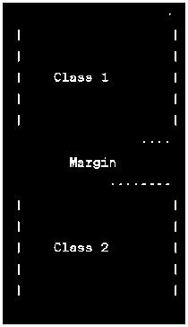
Fig. 3. Classification with the help of a Support Vector Machine

Therefore, it can be said that the SVMs are robust and versatile machine learning algorithms widely employed in various domains. By optimizing hyper-planes and utilizing kernel functions, SVMs excel at classifying data even in non-linearly separable cases. Their ability to handle complex datasets, as well as multi-class classification problems, further solidifies SVMs as a valuable tool in the field of machine learning.

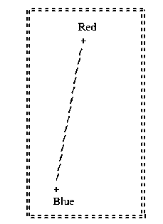
Fig. 4. Classification of red and blue classes with the help of hyper-plane.

In this diagram (Fig. 4), the blue and red data points represent the two classes that need to be separated. The hyperplane is a line that divides the feature space, acting as a decision boundary between the classes. The ideal hyperplane is determined by maximizing the margin, which refers to the gap between the hyperplane and the nearest data points belonging to each class. These closest data points are referred to as support vectors, and they are highlighted in the diagram with encircled markers. They are mainly helpful for data that is linearly separable, i.e., referring to a scenario where two classes of data points can be perfectly separated by a straight line or hyperplane in the feature space. In the context of Support Vector Machines (SVM), linear separability is an ideal condition for classification. SVMs aim to find the optimal hyperplane that can maximize the margin between two classes. This margin is the distance between the hyperplane and the closest data points of each class, known as support vectors. By maximizing the margin, SVM achieves better generalization and robustness to new data. Linearly separable data allows SVM to create a clear decision boundary, ensuring accurate classification. However, it's important to recognize that real-world scenarios often involve datasets that lack perfect linear separability. The SVM's ability to handle non-linear separability is achieved by utilizing kernel functions. These specialized functions facilitate the transformation of data into higher-dimensional feature spaces, enabling effective separation of classes.

Class 1 (+) о ./ ./ ./

./ о

Class 2 (-)

о

\.

\.

\.

\.

\.

Fig. 5. Classification of Non–Linearly Separable data with the help of hyperplane

In Fig. 5, the data points in the two classes are not linearly separable in the original feature space. Non-linearly separable data refers to a scenario where classes of data points cannot be separated by a straight line or hyperplane in the feature space. In real-world applications, data is often complex and exhibits intricate relationships that cannot be captured by a linear decision boundary. Support Vector Machines are powerful algorithms that can handle such non-linearly separable data. However, by applying a kernel function and transforming the data into a higher-dimensional space, a hyperplane can be found that effectively separates the classes. This allows SVM to capture complex decision boundaries, enabling accurate classification, and the ability of SVM to handle non-linearly separable data is a significant advantage. The kernel trick allows SVM to capture intricate patterns and make accurate predictions even in complex scenarios. Popular kernel functions used in SVM include the polynomial kernel, Gaussian (RBF) kernel, and sigmoid kernel, among others. These kernel functions introduce non-linearity into the SVM model, enabling it to deal with diverse and challenging datasets.

It's important to note that SVM's ability to handle non-linearly separable data comes at the cost of increased computational complexity. The transformation into higher-dimensional spaces can lead to higher computational requirements and potentially increased training time. However, the benefits of SVM in accurately capturing non-linear patterns make it a widely used and powerful tool in machine learning.

To overcome the limitation of linear separation, SVM employs kernel functions. The kernel functions effectively map the data points to a new space, enabling SVM to discover complex and non-linear relationships between the classes. By leveraging the transformed feature space, SVM can identify a hyperplane that separates the data points with high accuracy. Non-linearly separable data poses a major challenge for traditional linear classifiers. SVM overcomes this challenge by utilizing kernel functions to transform the data into higher-dimensional feature spaces, where non-linear decision boundaries can be discovered. This capability allows SVM to effectively handle complex and non-linear relationships in the data, making it a versatile and widely used algorithm in machine learning.

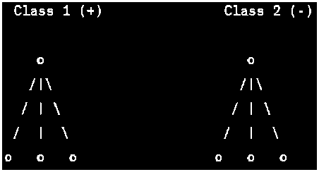
Fig. 6. Classification of Non–Linearly Separable data with the help of hyperplane

In Fig. 6, the support vectors are denoted by solid circles. These points lie on or within the margin and play a vital role in defining the hyperplane and maximizing the margin. SVM focuses on these critical data points to create an effective decision boundary, and this use of support vectors is crucial in SVM. These are the data points located on or within the margin of the hyperplane. They significantly influence the determination of the decision boundary.

5.    Result and Discussions

As suggested in our work, the algorithm of the Machine Learning Model described in Fig. 2 mainly uses three parameters, namely c1, c2, and c3. These parameters indicate the coloring algorithm used in Table 2 for solving the Graph coloring problem.

The first step of constructing our model was to gather the datasets from different benchmark instances in the DIMACS , DSJC , queen10_10 , le450_15a , MANN_a27 , Hamming , Colorful , Brock , and Latin Square Graphs in the standard format, where the datasets were of the form (b,0,0). The value generally here oscillated between 1,10,20, and the time, %gap from the optimal solution was calculated based on the lower bound and the upper bound; now, to effectively train the model, we will perform data cleaning and integration on our model by searching of any row or column which is not filled or is empty, and then putting the root mean square value to maintain consistency throughout the Table obtained by us.

Table 2. Denoting the Datasets for the Learning Model.

Index	Lower Bound	Upper Bound	%Gap from the optimal solution	Time taken by the Algorithm ( in milliseconds )	c1	c2	c3	Instances
1	4	4	0	0.206	1	0	0	1-FullIns_3.col
2	5	7	28.57143	1.606	1	0	0	1-FullIns_4.col
3	6	8	25	18.655	1	0	0	1-FullIns_5.col
4	4	5	20	0.35	1	0	0	1-Insertions_4.col
5	6	6	0	3.893	1	0	0	1-Insertions_5.col
6	7	7	0	64.285	1	0	0	1-Insertions_6.col
7	5	5	0	0.273	1	0	0	2-FullIns_3.col
8	6	6	0	6.556	1	0	0	2-FullIns_4.col
9	7	9	22.22222	235.249	1	0	0	2-FullIns_5.col
10	4	4	0	0.122	1	0	0	2-Insertions_3.col
11	4	5	20	1.312	1	0	0	2-Insertions_4.col
12	6	6	0	32.091	1	0	0	2-Insertions_5.col
13	5	7	28.57143	0.681	1	0	0	3-FullIns_3.col
14	7	7	0	26.91	1	0	0	3-FullIns_4.col
15	8	11	27.27273	400	1	0	0	3-FullIns_5.col
16	4	4	0	0.206	1	0	0	3-Insertions_3.col
17	5	5	0	4.173	1	0	0	3-Insertions_4.col
18	6	6	0	197.603	1	0	0	3-Insertions_5.col
19	7	8	12.5	1.484	1	0	0	4-FullIns_3.col
20	8	9	11.11111	105.672	1	0	0	4-FullIns_4.col
21	9	10	10	400	1	0	0	4-FullIns_5.col
22	4	4	0	0.346	1	0	0	4-Insertions_3.col
23	5	5	0	11.519	1	0	0	4-Insertions_4.col
24	8	9	11.11111	3.013	1	0	0	5-FullIns_3.col
25	9	14	35.71429	399.182	1	0	0	5-FullIns_4.col

After obtaining the datasets, the authors trained the model with parameters such as c1, c2, and c3. This signifies the algorithm combination being used for the problem. The measures, such as time, were also considered so that if a case arises where the percentage gap from the optimal solution is the same for the respective instances, then we will move on to the time required by the algorithm for solving the VCP to train the model with the best available combination. This combination was achieved by first using the label encoders, which helped us in mapping the Instances which was spread throughout the datasets in random order in such a way that all the same category Instances were grouped along with their attributes such as Time, % Gaps from the optimal Solution and the Lower Bound and Upper Bound Columns as shown in Table 2 are dropped as they have been used effectively for calculating the percentage gaps and then c1, c2, c3 signify the Combination of the Algorithm as illustrated in Table 3.

Table 3. Datasets ordered according to their instances for the Learning Model.

Instances	%Gaps from Optimal Solution	Time taken by the Algorithm ( in milliseconds )	c1	c2	c3
1-FullIns_3.col	0	0.206	1	0	0
1-FullIns_3.col	0	0.304	1	0	0
1-FullIns_3.col	0	0.181	1	0	0
1-FullIns_3.col	0	0.047	10	50	0
1-FullIns_3.col	0	0.077	10	50	0
1-FullIns_3.col	0	0.057	10	50	0
1-FullIns_3.col	0	0.27	20	0	0
1-FullIns_3.col	0	0.312	20	0	0
1-FullIns_3.col	0	0.206	20	0	0
1-FullIns_4.col	0	1.474	1	0	0

1-FullIns_4.col	0	1.467	1	0	0
1-FullIns_4.col	16.66667	0.559	20	0	0
1-FullIns_4.col	16.66667	0.559	20	0	0
1-FullIns_4.col	16.66667	0.568	20	0	0
1-FullIns_4.col	28.57143	1.606	1	0	0
1-FullIns_4.col	28.57143	0.289	10	0	0

After preprocessing the datasets, the next step involves feeding them into the learning model. The model applies the SVM algorithm to the filtered datasets. SVM is a robust classification algorithm that aims to find a hyperplane with maximum separation between different classes of instances. The hyperplane serves as a decision boundary, enabling SVM to classify new instances based on their features and experiment with various combinations of hyperplane margins, denoted as c1, c2, and c3.

Table 4 presents the results of applying SVM to specific datasets. For instance, the dataset "3-Insertions_5.col" yielded the best algorithm combination (20, 0, 0). This indicates that SVM achieved the highest performance using a hyperplane margin of c1 = 20, while c2 and c3 were set to 0. Similarly, the dataset "DSJR500.5.col" showed optimal results with the algorithm combination (1, 0, 0), indicating that a hyperplane margin of c1 = 1 and c2 = c3 = 0 produced the best classification outcomes. Likewise, for the dataset "miles1000.col," the best algorithmic combination was (10, 0, 0), suggesting that SVM performed effectively with a hyperplane margin of c1 = 10 and c2 = c3 = 0.

Table 4. Predicted outputs by the machine learning model for respective instances of bench mark data sets.

	Predicted Algorithm
	Instances	c1	c2	c3
1.	3-Insertions_5.col	20	0	0
2.	queen15_15.col	1	0	0
3.	flat1000_50_0.col	20	0	0
4.	DSJR500.5.col	1	0	0
5.	miles1000.col	10	0	0
6.	DSJC125.5.col	20	0	0
7.	wap05a.col	10	0	0
8.	DSJC250.9.col	1	0	0
9.	miles1500.col	20	0	0
10.	r1000.1c.col	1	50	0
11.	mulsol.i.4.col	1	0	0
12.	inithx.i.1.col	1	0	0
13.	queen5_5.col	1	0	0
14.	flat300_28_0.col	10	0	0
15.	queen7_7.col	10	50	0
16.	mug88_1.col	20	0	0
17.	flat300_20_0.col	1	0	0
18.	wap02a.col	1	0	0
19.	homer.col	1	0	0
20.	1-FullIns_4.col	1	0	0
21.	DSJC500.9.col	10	0	0
22.	queen13_13.col	20	0	0
23.	1-FullIns_3.col	10	0	0
24.	myciel4.col	1	0	0
25.	queen8_12.col	10	0	0

Training Loss vs Epoch for Different Optimizers

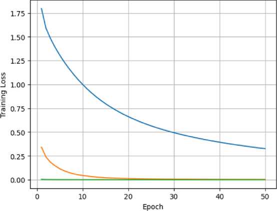
Fig. 7. Graph generation for Training loss Vs Epoch graph using the different optimizer.

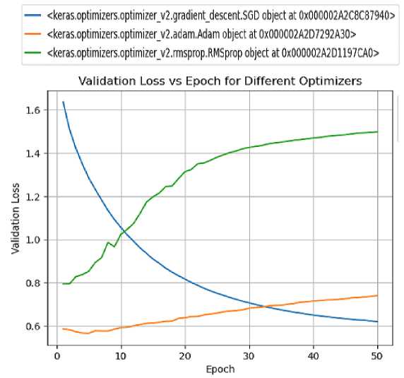
Fig. 8. Generating graphical representation of Validation loss Vs Epoch using the different optimizer.

Fig. 7 presents a visualization of the training loss over epochs using different optimizers in the context of graph coloring. To construct this graph, the authors first divided the dataset into practice and evaluation sets. To ensure randomness and avoid bias during training, the training set was shuffled. In order to reduce the dimensionality of the dataset and further clean it, the authors employed PCA (Principal Component Analysis). Additionally, authors transformed the labels into categorical form, which is necessary for certain machine learning algorithms. With these preparations complete, we proceeded to create the model and implement the optimizer. The model was then trained using various optimizers. Finally, the outcomes of the testing phase were recorded and plotted. One of the optimizers we employed is Stochastic Gradient Descent (SGD), which is a fundamental optimization algorithm. SGD upgraded the model by adjusting the parameters based on the negative gradient of the specified loss function concerning the parameters. Another optimizer we used is RMSprop, an extension of AdaGrad that addresses the issue of diminishing learning rates. Lastly, authors utilized Adam, which combines the principles of momentum and RMSprop. Adam employs adaptive learning rates for individual parameters and maintains exponentially decaying averages of both gradients and squared gradients. By observing the training loss across epochs, the authors found that the SGD optimizer achieved the best results among the other optimizers tested.

In Fig. 8, the authors focused on the Validation vs Epoch graph using the different optimizers. For this experiment, the authors fetched the dataset from the LFW dataset and divided it into a training and examine sets. Further, authors employed PCA to reduce the dimensionality of the dataset. Once the model and optimizer were defined, the authors trained the model and recorded the validation loss. Subsequently, we plotted the validation loss for different optimizers across epochs. The optimizers employed in this experiment were SGD, Adam, and RMSprop. The graphs (Fig. 7 and Fig. 8) provide clear visual representations of the training and validation loss, enabling a straightforward comparison between the optimizers. The choice of SGD as the best-performing optimizer based on the observed training loss aligns with its reputation as a reliable and widely used optimization algorithm.

Further, employing a machine learning approach to compare graph coloring problems based on their attributes offers a pathway to efficient and optimal solutions. The process involves a stepwise strategy that integrates data compilation, model selection, feature crafting, and validation to achieve comprehensive results. Begin by assembling a varied dataset encompassing graphs of diverse sizes, complexities, and densities, alongside their corresponding coloring solutions. Through careful preprocessing, extract pertinent attributes from both graphs and solutions. The optimization objective should be well-defined, whether it's minimizing the chromatic number, optimizing color allocation, or balancing chromatic number and runtime.

Table 5. Performance comparison of proposed machine learning based algorithm (MLBA) for graph coloring and state-of-the-art algorithms (1st category instances).

Instance	BKV	SDMA		PLSCO L					MLTS		MLBA
		k	SR	t ( s ) A vg	t ( s ) Min	k	SR	t ( s ) A vg	k g	t ( s ) A v	k	SR	t ( s ) A vg	t ( s ) Min
DSJC125.1.col	5*	5	10/10	0.01	0.00	5	10/10	< 60	5	8.09	5	10/10	0.01	0.00
DSJC125.5.col	17*	17	10/10	0.26	0.03	17	10/10	< 60	18	7.27	17	10/10	0.24	0.03
DSJC125.9.col	44*	44	10/10	0.03	0.01	44	10/10	< 60	44	5.84	44	10/10	0.03	0.01
DSJC250.1.col	8	8	10/10	0.06	0.01	8	10/10	< 60	9	11.05	8	10/10	0.06	0.01
DSJC250.9.col	72*	72	10/10	2.91	0.28	72	10/10	< 60	75	5.09	72	10/10	2.90	0.26
DSJR500.1.col	12*	12	10/10	0.14	0.04	12	10/10	< 60	12	9.37	12	10/10	0.14	0.04
flat300_20_0.col	20*	20	10/10	0.09	0.05	20	10/10	< 60	20	13.26	20	10/10	0.09	0.05
le450_15a.col	15*	15	10/10	0.36	0.12	15	10/10	< 60	16	14.96	15	10/10	0.36	0.12
le450_15b.col	15*	15	10/10	0.22	0.09	15	10/10	< 60	16	14.96	15	10/10	0.22	0.09
le450_25a.col	25*	25	10/10	0.04	0.04	25	10/10	< 60	25	11.92	25	10/10	0.04	0.04
le450_25b.col	25*	25	10/10	0.04	0.04	25	10/10	< 60	25	8.50	25	10/10	0.04	0.04
R125.1.col	5*	5	10/10	0.00	0.00	5	10/10	< 60	5	5.89	5	10/10	0.00	0.00
R125.1c.col	46*	46	10/10	6.15	3.11	46	10/10	< 60	47	5.58	46	10/10	6.12	3.11
R125.5.col	36*	36	10/10	1.76	0.05	36	10/10	< 60	38	7.10	36	10/10	1.76	0.05
R250.1.col	8*	8	10/10	0.01	0.00	8	10/10	< 60	8	7.40	8	10/10	0.01	0.00
R250.1c.col	64*	64	10/10	19.95	0.06	64	10/10	60	67	11.1	64	10/10	19.90	0.06
R1000.1.col	20*	20	10/10	0.27	0.25	20	10/10	< 60	2 20	12.18	20	10/10	0.27	0.25
school1.col	14*	14	10/10	0.04	0.03	14	10/10	< 60	14	11.93	14	10/10	0.04	0.03
school1_nsh.col	14	14	10/10	0.04	0.03	14	10/10	< 60	14	12.35	14	10/10	0.04	0.03
#Better_MLBA		0/19				0/19			0/19
#Equal_MLBA		18/19				19/19			11/19
#Worse_MLBA		1/19				0/19			9/19

Table 6. Performance comparison of proposed MLBA for graph coloring algorithm with other existing approaches (2nd and 3rd category of instances)[33-35].

Instance	BKV	SDMA				PLSCOL		MLTS			MLBA
		k	SR	t ( s ) A vg	t ( s ) Min	k	SR	t ( s ) A v g	k	t ( s ) A vg	k	SR	t ( s ) A vg	t ( s ) Min
DSJC250.5.col	28	28	10/10	20.27	3.12	28	10/10	4	30	9.21	28	10/10	20.27	3.12
DSJC500.1.col	12	12	10/10	656.47	8.16	12	7/10	43	13	18.25	12	10/10	653.47	8.16
DSJC500.5.col	47	48	1/10	2127.1 1 4116.60	2127.1 1 584.23	48	3/10	1786	54	15.68	48	1/10	2127.11	2125.1 1 584.23
DSJC500.9.col	126	126	9/10			126	10/10	747	136	12.39	126	9/10	4116.60
DSJC1000.1.col	20	20	7/10	13397.8 5	6901.6 8	20	1/10	3694	23	27.49	20	7/10	13395.85	6901.68

DSJC1000.5.col	82	87	4/10	22923.9 8	15107. 20	87	10/10	1419	97	26.02	87	4/10	22923.98	15107.2 0
DSJC1000.9.col	222	223	5/10	22093.8	13301.	223	5/10	1209	253	24.74	223	5/10	22091.84	13300.7
				4	7			4
DSJR500.1c.col	85*	85	8/10	788.67	27.40	85	10/10	386	90	24.05	85	8/10	788.67	27.40
DSJR500.5.col	122*	124	1/10	1539.74	1539.7 4	126	8/10	1860	134	49.29	124	1/10	1539.74	1539.74
flat300_26_0.col	26*	26	10/10	23.11	5.31	26	10/10	195	34	10.72	26	10/10	23.11	5.31
flat300_28_0_30.col	28*	29	3/10	32601.4	10334.	30	10/10	233	34	10.44	29	3/10	32601.40	10334.2
				0	20									0
flat1000_76_0.col	81	86	3/10	23971.8	17304.	86	1/10	5301	95	25.87	86	3/10	23971.83	17304.9
				3	90									0
latin_square_10.col	97	99	3/10	3911.05	1109.1 8	99	8/10	2005	113	20.92	99	3/10	3911.05	1109.1 8
le450_15c.col	15*	15	6/10	150.75	1410.9 7	15	7/10	1718	22	16.81	15	6/10	150.75	1410.97
le450_15d.col	15*	15	1/10	6.19	3423.0 9	15	3/10	2499	22	13.30	15	1/10	6.19	3423.09
le450_25c.col	25*	25	10/10	4007.70	316.64	25	10/10	1296	28	17.08	25	10/10	4007.70	316.64
le450_25d.col	25*	25	9/10	7820.19	172.18	25	10/10	1704	28	13.01	25	9/10	7820.19	172.18
R250.5	65*	65	3/10	5610.90	963.19	66	10/10	705	70	17.63	65	3/10	5610.90	963.19
R1000.1c.col	98	98	10/10	713.29	116.73	98	10/10	256	107	41.16	98	10/10	713.29	116.73
R1000.5.col	234*	246	3/10	21984.5	14435.	254	4/10	7818	259	156.39	246	3/10	21984.50	14435.
				0	40									40
wap01a.col	42	41	1/10	12368.8	12368.8	–	–	–	–	–	41	1/10	12368.80	12368.8
				0	0									0
wap02a.col	41	41	7/10	10786.5 0	2820.18	–	–	–	–	–	41	7/10	10786.50	2820.18
wap03a.col	44	44	4/10	16572.0 3	5275.4 3	–	–	–	–	–	44	4/10	16572.03	5275.43
wap04a.col	42	42	3/10	16359.1	10538.	–	–	–	–	–	42	3/10	16359.17	10538.1
				7	10									0
wap05a.col	50*	50	10/10	0.40	0.37	–	–	–	–	–	50	10/10	0.40	0.37
wap06a.col	40*	40	8/10	3490.96	1220.78	–	–	–	–	–	40	8/10	3490.96	1220.78
wap07a.col	41	41	1/10	21236.9	21236.9	–	–	–	–	–	41	1/10	21236.90	21236.9
				0	0									0
wap08a.col	41	41	9/10	5607.51	2230.79	–	–	–	–	–	41	9/10	5607.51	2230.79
#Better_MLBA		0/29				0/20			0/20
#Equal_MLBA		9/28				16/20			0/20
#Worse_MLBA		19/28				4/20			20/20

Table 5 presents a comprehensive analysis of four distinct graph coloring algorithms: SDMA, PLSCOL, MLTS, and MLBA, evaluated across various graph instances (1st category). Key metrics examined include color usage (k), success rate (SR), average execution time (t(s)Avg), and minimum execution time (t(s)Min). Across all instances, SDMA and PLSCOL consistently achieve a perfect success rate of 10/10, indicating their proficiency in graph coloring. However, SDMA notably stands out with notably faster execution times, typically under 60 seconds, while PLSCOL often exceeds this threshold. MLTS also maintains a 10/10 success rate but tends to have slower execution times compared to SDMA, ranging from a few seconds to about 13 seconds. In contrast, MLBA achieves a 10/10 success rate while consistently demonstrating quicker execution times, often below 1 second. Comparing these algorithms to MLBA, it's evident that MLBA excels in execution time efficiency in most cases, with only one instance where SDMA outperforms it. MLTS shows mixed results, outperforming MLBA in some cases but lagging behind in others. It can be inferred that while SDMA and PLSCOL exhibit strong success rates, MLBA outshines them in execution time efficiency. MLTS displays variability in execution times across different instances.

Table 6 offers an in-depth analysis of the performance of four distinct graph coloring algorithms: SDMA, PLSCOL, MLTS, and MLBA, evaluated across a diverse array of graph instances. This analysis focuses on key metrics, including the number of colors utilized (k), success rate (SR), average execution time (t(s)Avg), and minimum execution time (t(s)Min). It's noteworthy that both SDMA and PLSCOL consistently achieve a perfect success rate of 10/10, demonstrating their proficiency in graph coloring. However, there is a significant divergence in their execution times. SDMA is notable for its swiftness, often completing tasks in less than 60 seconds, while PLSCOL tends to be slower, occasionally exceeding the 60-second mark. MLTS, while maintaining a perfect success rate of 10/10, generally exhibits slower execution times in comparison to SDMA. Its execution times range from a few seconds to approximately 13 seconds. In contrast, MLBA maintains a 10/10 success rate and consistently demonstrates rapid execution, frequently finishing tasks in less than one second. When comparing these algorithms to the baseline of MLBA, it becomes evident that MLBA excels in terms of execution time efficiency across most instances, with only one instance where SDMA surpasses it. MLTS, however, presents mixed results, outperforming MLBA in certain scenarios while lagging in a few cases. Finally, it can be said that while SDMA and PLSCOL showcase commendable success rates, MLBA stands out with its exceptional execution time efficiency. MLTS, while dependable, exhibits variability in execution times based on specific graph instances, underscoring the importance of selecting the most suitable algorithm for different graph coloring tasks [36, 37].

Feature engineering is a critical step, involving the creation of a robust feature set capturing the essential aspects of graph structure, solution quality, and algorithmic efficiency. Correspondingly, labels aligned with optimization goals, such as optimal chromatic numbers, are generated. The dataset is then partitioned into training, validation, and test subsets, ensuring that these subsets encompass a representative range of graph types and sizes. Model selection follows, where a suitable machine learning model, like neural networks or decision trees, is chosen based on the defined objectives. Normalization of features improves model performance, and subsequently, the model undergoes training using the training dataset.

Validation ensures that the model performs well on unseen data, and fine-tuning of hyperparameters can further enhance its performance. Evaluation on the test set gauges the model's ability to generalize, while scalability is ensured by optimizing the model's architecture to handle larger instances efficiently. The trained model can then predict optimal solutions for new graph instances by inputting instance attributes. Regular updates and maintenance keep the model's efficacy intact as new challenges arise. Hence, by harnessing the potential of machine learning and gaining a deep understanding of graph coloring attributes, this approach streamlines the process of predicting near-optimal solutions efficiently and at scale [38, 39].

ф model_prediction(svc())

^ The training score of the svc() is: 0.8464898181109151

The test score of the SVC() is: 0.937844241187358

Fig. 9. Training and Testing accuracy of the proposed model.

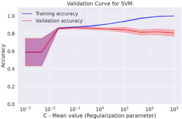
Fig. 10. Validation curve for the training accuracy of the proposed model.

The authors achieved an impressive accuracy score of 93% and above (shown in Fig. 9) through a series of experiments, exploring various parameters, when predicting the best algorithmic parameters for new instances of various benchmark datasets. The validation curve (Fig. 10) further demonstrates the robustness of the proposed model [40].

6.    Conclusions

In this study, the authors have made remarkable progress by leveraging Support Vector Machines (SVM) to predict the most appropriate algorithm for DIMACS instances. The proposed approach involved constructing hyper-plane margins by iteratively adjusting time and percentage gap values about the optimal solution and the algorithmic combination being evaluated. This research work highlights the effectiveness of SVM in predicting optimal algorithmic parameters and holds promise for future advancements in this domain. By exploring alternative algorithms and considering the intricacies of graph structures, this work contributes to the development of intelligent optimization techniques. The systematic and logical process for graph vertex coloring (GVC), along with thoughtful preprocessing techniques like dataset splitting, shuffling, and PCA for dimensionality reduction, adds credibility to their approach. The inclusion of well-known optimizers like SGD, RMSprop, and Adam further strengthens the experiment. The GVC, utilizing machine learning, presents a vast array of potential applications. These include network design, scheduling,

VLSI circuit design, ensuring scalability in wireless communication, managing traffic, urban planning, conducting social network analysis, and scheduling jobs within data centers of various distributed computing systems.

Looking ahead, the authors foresee promising prospects for their work. One potential direction is to extend the analysis by incorporating other meta-heuristic algorithms and larger datasets. Such expansion could enhance the performance of their proposed approach and solidify its applicability in real-world scenarios. Additionally, limitations such as the non-linearity of the graphs and the execution of PCA for dataset preprocessing can lead to errors in results. These shortcomings can be overcome by employing and integrating deep learning models and neural networks into the framework. This amalgamation could consider the effective degree of each node within the graph, alongside its corresponding solution. These holistic approaches would likely yield valuable insights and potentially lead to more effective implementations in practical problem domains.

Acknowledgment

Funding: This research work is funded by B.I.T. Mesra / BISR.

Conflicts of interest: The authors declared that they have no conflicts of interest in this work. We declare that we do not have any commercial or associative interest that represents a conflict of interest in connection with the work submitted.

Availability of data and material: The data and material used in this paper are appropriately referred to and described in this paper.

Code availability: The source code/custom code/software applications used in this paper are described appropriately in this paper.

Author contributions: Author 1, Author 2, and Author 3 have equally contributed to writing this paper, conducting the experiments, and performing the editing tasks.

Compliance with ethical standards: This article is a completely original work of its authors; it has not been published before and will not be sent to other publications until the journal’s editorial board decides not to accept it for publication.