A Packet Routing Model for Computer Networks

Author: O. Osunade
Journal: International Journal of Computer Network and Information Security(IJCNIS) @ijcnis
Article in issue: 4 vol.4, 2012.
Free access
The quest for reliable data transmission in today’s computer networks and internetworks forms the basis for which routing schemes need be improved upon. The persistent increase in the size of internetwork leads to a dwindling performance of the present routing algorithms which are meant to provide optimal path for forwarding packets from one network to the other. A mathematical and analytical routing model framework is proposed to address the routing needs to a substantial extent. The model provides schemes typical of packet sources, queuing system within a buffer, links and bandwidth allocation and time-based bandwidth generator in routing chunks of packets to their destinations. Principal to the choice of link are such design considerations as least-congested link in a set of links, normalized throughput, mean delay and mean waiting time and the priority of packets in a set of prioritized packets. These performance metrics were targeted and the resultant outcome is a fair, load-balanced network.
Network communications, routers, priority control scheme, routing model, traffic analysis
Short address: https://sciup.org/15011072
IDR: 15011072
Text of the scientific article A Packet Routing Model for Computer Networks
Published Online May 2012 in MECS
Computer networks can be seen as the collection of interconnected and simultaneously autonomous computer systems mainly for the purpose of sharing computer resources and communication [1, 2].The recrudescence of computer networks and its attendant unprecedented advantages led to its increasing use in today’s communication system. It offers reliable data, voice, and video communication, which is the prime expectation of its users at both ends of the network.
Computer networks can span local areas such as buildings to form Local Area Networks (LAN) or wide areas such as countries forming Wide Area Networks (WAN). The Internet is the most popular type of computer network because it gives reliable and efficient transfer of information – data, voice, and video. The quest for reliable data transfer necessitated the concept of routing, which is the process of finding a path from the source to a destination system in the network. It allows users in the remotest part of the world to get to information and services provided by computers anywhere in the world. Routing is what makes networking and internetworking at large magical. It allows voice, video and data from different location in the world to be sent to multiple receivers around the world. The concept of routing addresses such intricacies like selection of paths that span the world, adaptation of routing system to failed links, path selection criteria such as least delay, or least cost or most available capacity links. However, the performance of routing depends on the routing algorithms adopted [3].
Routing is accomplished by means of routing protocols that establish mutually consistent routing tables in every router or switch controller in the network. Routers build routing tables that contain collected information on all the best paths to all the destinations that they know how to reach [4]. A routing table contains at least two columns: the first is the address of a destination endpoint or a destination network, and the second is the address of the network element that is the next hop in the “best” path to this destination. When a packet arrives at a router, the router consults the routing table to decide the next hop for the packet [5].
In the face of the importance of routing, several routing techniques have been developed to improve packet receipt and packet delivery. A good routing technique however, is expected to be simple, robust, correct, flexible, stable and converge rapidly.
-
II. RELATED WORKS
Searching a suitable route (or path) for a packet transmission from a source node to its destination node is one of important issues in routing. A node is a host computer, a personal computer, a workstation or something like those. To choose any route, routing protocols adopt routing metrics which according to [6, 7], include minimum hop criterion, least cost criterion, and minimum delay.
The simplest is the minimum hop criterion, which specifies the path taken by packets through the least number of nodes. It is an easily measured criterion and it minimizes the consumption of network resources. The least cost criterion has a cost associated with each link, and, for any pair of attached nodes, the route through which the network accumulates the least cost is sought. This suggests that the least cost should provide the highest throughput and minimizes delay. The minimum delay is such that routes are dynamically assigned weights based on the traffic on those routes and routing tables are repeatedly revised such that paths with close to minimal delays are chosen [7]. The first two routing metrics are the major performance criteria found in routing out of which least cost is more common because it is found to be more flexible compared to others.
Routing is accomplished by means of routing protocols that establish mutually consistent routing tables in the router (or switch controller) in the network. Routing protocol is more of a standard method of implementing a particular routing algorithm. Pertinent to routing protocols are routing tables. A routing table contains at least two columns, the first is the address of a destination endpoint or a destination network, and the second is the address of the network element that is the next hop in the “best” path to this destination. Whenever a call-setup packet or any packet arrives at router, the router or switch controller consults the routing table to decide the next hop for the packet. This essentially expresses the significance of routing tables and ultimately the essence of routing protocols.
A desirable routing protocol must satisfy several mutually opposing requirements amongst which are the following:
-
• Minimizing routing table space: One would like routing tables to be as small as possible, so that we can build cheaper routers withy small memories that are more easily looked up. The larger the
routing table, the greater the overhead in exchanging routing tables. It is required that routing table grows more slowly than the number of destinations in the network.
-
• Minimizing control messages: Routing protocols require control message exchange. These
represent an overhead on system operation and should be minimized.
-
• Robustness The worst thing that could occur within a network or internetwork is to misroute packets, so that they never reach their destination.
-
• Using optimal paths To the extent possible, a packet should follow the “best” path from a source to its destination.
Pertinent to note, these entire requirements may not be practicable to implement in a single protocol. They represent trade-offs in routing protocol design. A protocol for instance may trade off robustness for a d ecrease in the number of control messages and routing-table space for slightly longer paths .
Common Routing Protocols
Routing protocols enable routers within a network to share information about potential paths to specific hosts within that network. Examples of routing protocols include Routing Information Protocol (RIP-v1 and RIP-V2 being the latest), Open Shortest Path First (OSPF), Interior Gateway Routing Protocol (IGRP). Each routing protocol has its own unique features, benefits, and limitations.
Protocols in this wise can either be interior or exterior. Exterior protocols determine routing between entities that can be owned by mutually suspicious domains. Exterior protocols configure border gateway (that is, gateways that mediate between interior and exterior routing) to recognize a set of valid neighbours and valid paths. The protocols commonly used for exterior routing are the Exterior Gateway Protocol (EGP) and the Border Gateway Protocol (BGP).
Interior protocols are largely free of the administrative problems that exterior protocols face. Interior routing protocols typically hierarchically partition each AS into areas. Two protocols are commonly used as interior protocols. These are Routing Information Protocol (RIP) and the Open Shortest Path First protocol (OSPF).
Routing Algorithms
Routing Algorithms are systematic schemes capable of maintaining information about the network. They derive routing tables from this information thereby keeping track of network addresses and the paths through which packets can be routed. The two fundamental routing algorithms in packet-switched networks are Distance vector routing algorithm (DVA) and Link state routing algorithm (LSA) [4]. Both algorithms assume that a router knows the address of each neighbour and the cost of reaching each neighbour node. The cost in this case measures quantities like the link’s capacity, the current queuing delay, or a per-packet charge. They both keep the global routing information, that is, the next hop to reach every destination in the network by the shortest path (or least cost).
In a distance-vector algorithm, a node tells its neighbours its distance to every other node in the network. Here, it’s assumed that each router knows the identity of every other router in the network but not necessarily the shortest path to it. Each router maintains a
distance vector
, that is, a list of
In a link-state algorithm, a node tells every other node in the network its distance to its neighbours. The philosophy in link-state routing algorithms is to distribute the topology of the network and the cost of each link to all the routers. Each router independently computes optimal paths to every destination. This suggests that if each router sees the same cost for each link and uses the same algorithm to compute the best path, the routes are guaranteed to be loop-free. A prominent link-state algorithm is the Dijkstra’s algorithm [7].
All these make both routing algorithms distributed and suitable for large internetworks controlled by multiple administrative entities.
Performance Assessment and Evaluation of LSA and DVA
-
• Conventionally, Link-state algorithms are more stable because each router knows the entire network topology. On the other hand, if the network is so dynamic that links are always coming up or going down, then these transients can last for a long time, and the loop-free property is lost. Thus, one should not prefer link-state protocols for loop-freeness alone.
-
• LSA can carry more than one cost. Thus each router can compute multiple shortest-path trees, one corresponding to each metric. Packets can then be forwarded on one of the shortest-path trees.
-
• LSA may carry a delay cost and a monetary cost that allow every router to compute a shortest– delay tree and a lowest-monetary-cost tree.
-
• LSA is preferred to distance-vector algorithms because, after a change, they usually converge faster. But it is not clear if this actually holds if one uses a distance-vector algorithm with triggered updates to ensure loop-freeness and therefore absence of counting to infinity plaguing DSAs.
-
• DSA has two advantages over link-state algorithms. First, much of the overhead in linkstate routing is in the elaborate precautions necessary to prevent corruption of the LSP database. This could be avoided in DVA because they do not require that nodes independently compute consistent tables. Secondly, DVA typically require less memory for routing tables than do link-state protocols. This advantage could disappear if one uses path-vector-type distancevector algorithms.
Since there is no clear winner, both DVA and LSA are commonly used in packet-switched networks.
EXISTING SCHEMES
-
i. Dijkstra’s Algorithm
This algorithm according to [8, 9] requires that all link lengths (or cost) are non-negative, which is the case for most network applications. The basic idea of this algorithm is to find the shortest paths from a given node (called the source) to all other nodes of the network in order of increasing path length. At step k, k = 1,2…N-1, we obtain the set P of k nodes that are closest to the source node 1, where N is the number of nodes in the network. At step k+1, we add a new node to the set P, whose distance to the source is the shortest of the remaining nodes not included in the set P. Let D(i) denote the distance from the source to node i along the shortest path traversing nodes within the set P, and ℓ(i, j) denote the length of the link from node i to node j, where D(i) (or ℓ(i, j)) is equal to ∞ if no such path (or link) exists.
Initially, P = {1}, D(1) = 0 and D(j) = ℓ(1, j) for j ≠1.
The algorithm can be presented as follows:
-
• Step 1, find the next closest node i Є P such that D(i) = min D(j), j Є P.
Set P = P U {i}. If P contains all nodes, then the algorithm is complete.
-
• Step 2, for all the remaining nodes j Є P, update the distances.
D(j) = min (D(j), D(i) + ℓ(i, j)). Go to step 1
Since each step in Dijkstra’s algorithm requires a number of operations proportional to |N|, and the steps are iterated |N-1| times, the worst case computation is O(|N|2) [10].
-
ii. Bellman-Ford Algorithm for Shortest Paths
This algorithm requires that the lengths (or costs) of all cycles are non-negative. The basic idea of the algorithm is to iterate on the number of arcs in a path. At step k of the algorithm, D(i) records the distance from node i to the destination node 1 through the shortest path that consists of at most k arcs, where D(i) is equal to ∞ for i ≠ 1. The algorithm can be presented as follows for all the nodes i ≠ 1.
-
• Step 1, find the adjacent node w of the node i such that
-
• D(w) + ℓ(i,w) = min j ( D(j) + ℓ(i,j)) where the minimization is performed over all nodes j that are neighbours of node i.
-
• Step 2, Update the distance, D(j) = D(w) + ℓ(j,w). Repeat this process until no changes are made.
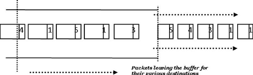
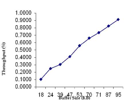
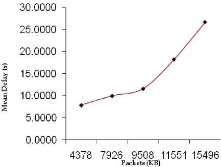
In the worst-case, N iterations have to be executed, each of which involves N-1 nodes, and for each node there are no more than N-1 alternatives for minimization. Therefore, a simple upper bound on the time required for the Bellman-Ford algorithm is at most O(N3), which is considerably worse than the time required by Dijkstra’s algorithm. However, we also show that the Bellman-Ford algorithm can be reduced to O(hA), where A is the number of links in the network and h is the maximum number of links in a shortest path. In a network that is not very dense, we have A< Generally speaking, efficiently implemented variants of the Bellman-Ford and Dijkstra’s algorithms appear to be equally competitive. iii. Floyd-Warshall Algorithm For Shortest Paths This algorithm finds the shortest paths between all pairs of nodes together and requires that the lengths (or costs) of all cycles are non-negative [11]. The basic idea of the algorithm is to iterate on the set of nodes that are allowed as intermediate nodes. At step k, D(i,j) records the distance from node i to node j through the shortest path with the constraint that only nodes 1,2, …,k can be intermediate nodes. The algorithm can be presented as follows. Initially, D(i,j) = ℓ(i,j) for all i,j, i≠j for k= 1,2,…,N, D(i,j) = min(D(i,j), D(i,k) + D(k,j)), for all i≠j. Since each of the N steps must be executed for each pair of nodes, the time required for the Floyd-Warshall algorithm is O(N3). PERFORMANCE METRICS The following metrics will be used to measure the performance of the multiple-access (routing) scheme: Normalized Throughput or Goodput This is the fraction of a link’s capacity devoted to carrying non-retransmitted packets. Goodput excludes time lost to protocol overhead, collisions, and retransmissions. For example, consider a link with a capacity of 1Mbps. If the mean packet length is 125bytes, the link can ideally carry 1000packets/s. However, because of collisions and protocol overheads, a particular multiple-access scheme may allow a peak throughput of only 250 packets/s. The goodput of this scheme, therefore, is 0.25. An ideal multiple-access protocol allows a goodput of 1.0, which means that no time is lost to collisions, idle time, and retransmission. Real-life protocols have goodputs between 0.1 and 0.95. Fairness It’s intuitively appealing to require a multiple-access scheme to be “fair”. There are many definitions for fairness. A minimal definition, also called nostarvation, is that every station should have an opportunity to transmit within a finite time of wanting to do so. A stricter metric is that each contending station should receive an equal share of the transmission bandwidth. III. PROPOSED SCHEME The objective of this model is to provide a typical framework for routing in a typical computer network. The model considers a case of N users contending for bandwidth over a known number of links between the source and the destination with the sole aim of routing packets to the desired destination. Each user routes at a fixed data transfer rate. The development of the routing framework is based on the following components: • Source Packet Generator (Packetizer) • Routing Device and the Queuing System • Links and Bandwidth Allocation • Time-based Bandwidth Generator • Destination Figure 1 is the schematic diagram of the proposed routing model. Each of these components is made up of subcomponents which are subjected to mathematical exposition and manipulations. The Packetizer Packets are sequences of bits of varying size. They are meant to be routed over some available links in the network using certain distinct metrics such as link cost, waiting time or delay and minimum hop. The packetizer generates sequence of random bits of varying size in order to simulate the routing of packets over available links to the targeted destination. A special consideration is given to the fact that packets so generated are assumed to be sent out by N users. Routing Device and the Queuing System At the routing device, a table called the decision table or routing table is maintained to ascertain the address of a destination endpoint or a destination network and the address of the network element that is the next hop in the best path to this destination. In this model, the best path to the destination will be evaluated by considering the: • Least cost link over the available set of links and • Least-congested link provided the link is available for packet transfer The cost over each link will be evaluated using the average link cost equation in a typical packet traffic regime. Average cost fℓ (λℓ) over each link ℓ is given as fℓ (λℓ) = aℓλℓ = R/(Σ 1/am), m= 1,2…M (1) Each packet generated is routed to the desired destination through the most desirable set of links. The most desirable link will later be determined using a specific metric. If there is no packet to send, nothing is sent on the link. When a packet is ready, and the link is idle or capable of admitting the size of the packet, then the packet can be sent immediately. The concern of this component of the model development is that, if the link is very busy, that is, another packet is currently being transmitted or the bandwidth is so choked up or the link is so congested that it cannot accommodate the on-coming packets, then the packet must wait in a buffer administered by a queuing system until the previous block of packet has been completely transmitted. The queuing theory as a mathematical concept will be used to express the idea of resource contention. Packets awaiting bandwidth allocation must wait in the queue and tagged a priority level until they are routed and dropped from the queueing system. In modelling the queuing system, the case of Kendall’s M/G/1 queue is adopted. The first letter “M” species the inter arrival time distribution and the second letter “G” specifies the service time distribution, while the third letter specifies the number of servers (in this case “1”) [12]. Kendall explains M/G/1 queue as being characterized by an infinite buffer queue in which case arrivals occur according to a Poisson process with rate λm, service times have independent general distribution where inter-arrivals and service times are independent. Since M/G/1 queue offers an infinite buffer, then it follows logically that packet drop or packet loss due to exhausted buffer is eliminated. Poisson distribution process for packet arrivals is given as, a (k) = (λk/k!) e-λ (2) k = arrivals in one time slot λ = arrival rate per time slot General distribution process for packet service times is given as an arbitrary probability density function fy(У)(3) The first two moments of the service time are sufficient to obtain the average packet delay and system occupancy [13]. β1m = E(У) = 1/μ(4) β2m = E(У2) = 2/μ(5) An important expression in the analysis of M/G/1 queues is the Pollaczek-Khinchin formula, which related the average system occupancy to the arrival and service parameters. Average system occupancy, that is, the average number of packets in the system and the average packet delay are as follows, E(N) = ρ + {(λ2 E(У2) / 2(1 – ρ)} (6) E(T) = 1/ μ + {(λ E(У2) / 2(1 – ρ)} (7) Queuing system notations and definitions • M = Parallel links between the source and the destination • N = Users sending packets from source to destination • Ri = Total rate of transmission required by user i • λm = The total rate of packet sent over link m, that is, Σi λim • μ = the average number of packets that are served per unit time. • 1/ μ = the average time a packet spends in the server. • ρ = λ/μ, is the server utilization. PRIORITY CONTROL SCHEME In real life networks, signals such as data, voice and video arrive in varying priorities depending on the type of service e.g. real time, time sharing and the type of message being sent. For instance, a continuous message like video and voice signals will carry higher priority than data. Queuing systems with priority classes are divided into two types: Pre-emptive priority and Non-pre-emptive priority. In pre-emptive priority discipline, whenever a higher priority packet arrives while a lower priority packet is in service, the lower priority packet is pre-empted and is taken out of service without having his service completed [14]. In this case, the pre-empted packet is placed back in the queue ahead of all packets of the same class. Under the non-pre-emptive priority discipline, once the service of any of the packet is started, it is allowed to be completed regardless of arrivals from higher priority class. In this model framework however, non-pre-emptive priority, which is more appropriate for packet transmission is adopted. Packets arrive at the buffer in varying priority levels. The highest priority packet is hitherto marked 1 and the lowest priority packets marked 5. Figure 2 shows a flow of prioritised chunks of packets through the buffer. IN BUFFER Flow of Packets _ . , - , , J Increasing order of packet priority leaning the buffer Packets from Flow of Packets Figure 2: Schematic Diagram of Priority Control Scheme Links and Bandwidth Allocation Links are routes through which packets are forwarded to the destination network. The buffer comes in between the source and the destination network. It is often implemented at the routing device. In this model development, special consideration will be given to links availability and congestion by evaluating bandwidth capacity at any given point in time. This factor prompts the functional definition of the succeeding phase. Time-Based Bandwidth Generator In order to simulate the selection of the most desirable link or route in routing packets to their destination, a time-based bandwidth generator will be used. The time-based bandwidth generator generates random numbers typical of bandwidth sizes or capacity over a known range of time, 0 ≤ t ≤ T. This suggests that at any given time t, there will always be a known bandwidth capacity B Mbps such that the available bandwidth determines when to route packets over the link and the size of packet that can be accommodated over any given link at any point in time. Destinations Considering the framework so designed, that is, a general-topology network with end-to-end connection of source and destination linked by several routes and several hops, packets are only routed from the source network (and not node) to the destination network before they are later picked up and transmitted to the individual nodes in form of frames. A single destination unit is assumed for this work. IV. PERFORMANCE ANALYSIS AND RESULTS In order to adhere to the performance metric specified by the methodology, the simulation endeavours to effect “fairness” into the network by way of load balancing the incoming packets over the set of available links. The load balancing metric ensures that within some time interval, all the available links are serviced such that no link is relatively idle and none of the link is relatively congested. Tables 1, 2 and 3 show the relationship existing between Throughput (Kbps) and Buffer Size (KB), Mean Delay(s) and Packet Size (KB) and Mean Waiting Time (s), Mean Delay (s) and Arrival Rate (Kbps) respectively. Table 1: The Relationship between Throughput (Kbps) and Buffer Size (KB) Buffer Size (KB) Throughput (%) 18 0.1032 24 0.2489 39 0.3045 47 0.4112 53 0.5589 70 0.6626 71 0.7360 87 0.8262 95 0.9144 Table 2: The Relationship between Mean Delay(s) and Packet Size (KB) Packet Size (KB) Mean Delay (s) 4378 7.9140 7926 10.0000 9508 11.6291 11551 18.2734 15496 26.6667 Table 3: The Relationship among Mean Waiting Time (s), Mean Delay (s) and Arrival Rate (Kbps) Arrival Rate (Kbps) Mean Waiting Time (s) Mean Delay (s) 31 1.8779 7.3779 68 5.4585 10.9585 77 6.7116 12.2116 105 12.4882 17.9882 121 18.1771 23.6771 Figure 3 shows the relationship between the network throughput and the system buffer size. As the buffer size increases, the network throughput increases and approaches 1.0. This relationship typifies an increasing rate of network throughput but the maximum cannot be reached due to some inhibiting factors such as interference and other exogenous factors. Figure 3: The graph of Throughput (Kbps) against Buffer Size (KB) Figure 4 shows the relationship between the mean delay in the system and the packet. As the total number of packets in the system increases at any point in time, there is a consequential induction of delay into the system. This delay is essentially caused by a resultant congestion in the network. Figure 4: The graph of Mean Delay(s) against Packet Size (KB) Figure 5 is a dual-purpose graph that shows that as the packet arrival rate (λ) at the buffer increases, in this case, an M/G/1 queue as specified by the simulation model, packets easily get congested in the system thereby causing an upward movement in the mean delay and mean waiting time of packets in the system. The graphs are dynamically generated by the simulation code so as to reflect the behaviour of the system at any given point in time. The research endeavours of Dijkstra cannot particularly be outwitted but a level of parallel output is obtained by the analysis of how the network incurs its mean waiting time, mean delay and overall throughput. Dijkstra’s algorithm is found to possess a very high throughput by virtue of the minimized mean delay incurred by its implementation. The discrepancy found between the existing and the proposed schemes is due to the residual service time characterising the proposed scheme. The residual service time is brought about by the use of prioritised packets. If it were to be a general class of packets, then the issue of residual service time wouldn’t have been necessitated. It is however note worthy, that over the existing scheme, a very “fair” network load balancing is maintained in the proposed scheme. In addition, the tendency of packet loss is duly minimised by the M/G/1 queueing system implemented. The crop of merits and demerits of the proposed scheme thus, leaves room for further work and improvement. V. CONCLUSION The research work has been an expository one into the many issues in data communication. The proposed routing model is meant to offer an improved means of routing or transferring data from emerging sources to their correct destination. To a considerable extent, the model implemented exhibited good results for the performance metrics targeted such as fairness, load balancing, normalized throughput and a manageable mean delay in the system.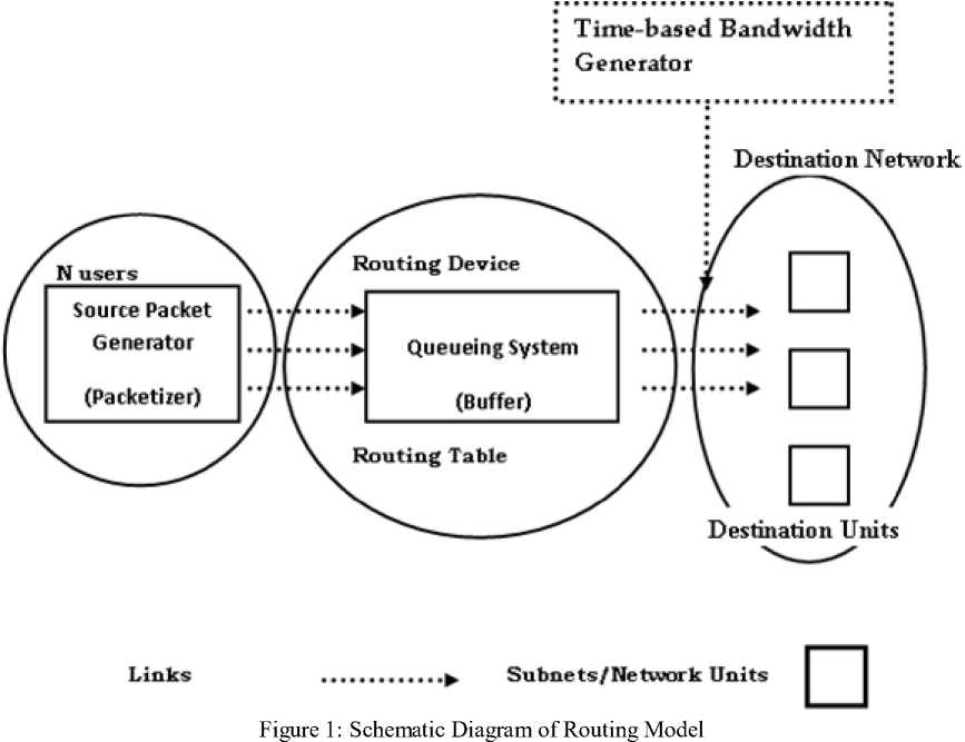
References A Packet Routing Model for Computer Networks
- Ray Horak (2000). Communications Systems and Networks, M & T Books, An imprint of IDG Books Worldwide, Inc., California.
- Tittel E., Hudson K. and Stewart J.M. (2000). Networking Essentials. Exam 70-058. 3rd Edition. Coriolis. USA.
- Yashpaul Singh E.R., and Swarup A. (2009). Analysis of Equal cost Adaptive Routing Algorithms using Connection-Oriented and Connectionless Protocols. World Academy of Science, Engineering and Technology 51 2009, pp.299-302.
- Halabi, S. and McPherson, D. (2000). Internet Routing Architectures. 2nd Edition. CISCO Press. Indianapolis, USA.
- Malhotra, Ravi (2002). IP Routing. First Edition. O’Reilly & Associates, Inc. USA.
- Lonnberg Jan, 2002. Routing algorithms. Based on G. Tel: Introduction to Distributed Algorithms, chapter 4.Retrieved online at www.tcs.hut.fi/Studies/T-79.192/.../lonnberg_slides_021002.pdf- Routing algorithms
- Mak R. H. (2011). Routing Algorithms 1. ISE 435: Distributed Algorithms in Network Communication. Retrieved online at www2.kinneret.ac.il/mjmay/ise435/435-Lecture-12-Routing1.pdf
- Joyner, D., Nguyen, M. V. and Cohen, N. (2010). Algorithmic Graph Theory. Version 3.0 (Electronc version). Available at “graph-theory-algorithms-book.googlecode.com”
- Varvarigos E.M. and Yeh C.H. (1999). Networking Routing Algorithms, In: Wiley Encyclopedia of Electrical and Electronics Engineering. Webster J.G. (ed), John Wiley & Sons, Inc., New York, Vol. 14, pp.222 – 227.
- Tommiska Matti and Skytta Jorma (2001). Dijkstra’s Shortest Path Routing Algorithm in Reconfigurable Hardware. Proceedings of the 11th Conference on Field-Programmable Logic and Applications (FPL 2001). Belfast, Northern Ireland, UK, 27-29 August 2001, pages 653-657.
- Lonnberg Jan, 2002. Routing algorithms. Based on G. Tel: Introduction to Distributed Algorithms, chapter 4.Retrieved online at www.tcs.hut.fi/Studies/T-79.192/.../lonnberg_slides_021002.pdf- Routing algorithms
- Adan, I. and Resing, J. (2002). Queueing Theory. Department of Mathematics and Computing Science Eindhoven University of Technology, the Netherlands.
- Azizoğlu, M. and Barry, R.A. (1999). Network Performance and Queueing Models, In: Wiley Encyclopedia of Electrical and Electronics Engineering. Webster J.G. (ed), John Wiley & Sons, Inc., New York, Vol. 14, pp.204 – 214.
- Chen, F. (2006). Admission Control and Routing in Multi-priority Systems. A dissertation University of North Carolina at Chapel Hill.
