A Proposed Technique for Solving Scenario Based Multi-Period Stochastic Optimization Problems with Computer Application

Stochastic programming (SP) is a special kind of mathematical programming that deals with uncertainty [1]. It is closely related to linear programming (LP) problem. LP is a deterministic problem. When some or all of the parameters of LP contains uncertainty then it is called SP. The beginning of SP dates back to the 50’s and 60’s of the last century. G. B. Dantzig first formulated the general problem of LP with uncertain data [8] and he is considered as a pioneer to establish SP as a branch of mathematics. The main advantage of SP is that it can estimate the probability of occurring different scenarios for respectable uncertainty [8]. It extends the scope of

* Corresponding author. Tel.: +8801927220703

linear and non linear programming problems by including probabilistic or statistical information in different parameters. In real life, there are lots of applications of SP [16]. It has a great implementation in production, supply chain, scheduling, gaming, environment etc. Fleet management model by B. Powell and H. Topaloglu [13], Model for Network Recourse Utilization by Julia L. Higle and Suvrajeet Sen [16] are some of the most popular and renowned applications of SP.

Due to uncertainty number of variables and conditions in SP problems are comparatively more than any LP problems. So it is very difficult to solve SP problems by hand calculations. To solve these large scale problems decomposition techniques are more applicable. By these techniques large scale optimization problems can be solved by decomposing into sub-problems and a master problem. In this paper, we have developed a technique for solving SP problems. We have used idea of decomposition based pricing (DBP) method.

In Bangladesh, Super shop markets are getting popularity day by day like many other developed countries. Due to the management system and quality of products peoples are getting interested about super shops. There are around thirty super shops in Dhaka, which is the capital of Bangladesh and they have also many branches in other cities around the country.

In this paper, we have developed a real life stochastic model by collecting data from a super shop market. It is very difficult to analyze the model by hand calculation because it is a large scale problem. That’s why we develop a computer code by using AMPL to analyze the model.

Rest of the paper we have organized as follows. We first discuss some preliminaries and basic definitions in Section 2. Then we have focused on some existing solution procedures of SP in Section 3. After that, we have presented our developed model in Section 4 by collecting data from a super shop market of Bangladesh and presented a stochastic formulation of this model in Section 4.1. In Section 5, we have presented the algorithm of our developed technique on perspective of our model. Then we have presented a short discussion about the AMPL code we developed and then presented a comparison of profits obtained in different periods in Section 5.1 and 5.2 respectively. Finally, we have drawn a conclusion about our work and presented references which we have used.

• 2.    Preliminaries

• 2.1.    Stochastic Programming (SP)

In the current section, we define stochastic programming (SP) problems, scenario based SP, basic ideas of decomposition techniques. We clarify the meaning of sub-problem and master problem used in decomposition techniques and the steps of decomposition based pricing (DBP) technique. We have discussed these as follows.

Consider the following linear programming (LP) problem [11].

T

Maximize (or Minimize) z = c x(1)

subject to

Ax = b(2)

x > 0

The m x n matrix A= (a,,) —  — is the coefficient matrix of the equality constraints (2), v ij'i=1,m,j=1,n                                                               q      y b = (b1, b2,......, bm ) ) is the right hand side vector of the constraints (2), the components of c are the profit factors and, x = (x ,x ,......, x )T ∈ Rn is the vector of variables, called the decision variables and x ≥ 0

are called non-negative restrictions.

When some or all of the parameters of LP problem contains uncertainty then it is called SP problem. A mathematical formulation of SP problems has given below [4].

T

maximize (or minimize) z = cω xω(4)

subject to

Axω = b(5)

xω ≥ 0

Here we have considered that the profit factor c in equation (4) contains uncertainty for different scenarios ω and x represents corresponding stochastic decision variables. There are different types of SP. In this paper, we mainly impose our attention to scenario based SP. In the next section, we discuss about scenario based SP.

• 2.2.    Scenario Based SP

  A scenario for a stochastic model is a collection of outcomes for all the stochastic events taking place in the model, along with the associated probability of the scenario to occur. Khan and Weiner (1967) [14], probably first originated scenario analysis, defined a scenario as a hypothetical sequence of events constructed to focus on casual processes and decision points.

There are different types of SP problems. Expected value problem, Wait and see, Chance constrained problem etc are some of them [3]. In this paper, we have worked with scenario based SP. SP associated with scenarios for respectable uncertainties inserted in any or all parameters is called scenario based SP. A mathematical formulation of this type SP has given below.

T

maximize (or minimize) z = p c x(7)

subject to

Axω ≤ b(8)

xω ≥ 0

In this problem, p in equation (7) is representing the probability for scenario ω , c^T is for profit factor obtained for different scenarios ω and x are the corresponding stochastic decision variables for scenarios ω . Here we have considered profit factor as an uncertain parameter. Uncertainty can be raised in A or b or in both at the same time. In the next section, we discuss about the basic idea of decomposition technique.

• 2.3.    Decomposition, Sub-problem and Master Problem

Decomposition is a solution procedure of large scale LP problems. It started working by decomposing the whole problem into sub-problems and a master problem. There are several types of decomposition techniques in use. Dantzig-Wolfe decomposition, Bender’s decomposition [2], triangular decomposition etc are some of them. We have discussed decomposition technique, sub-problem and master problem briefly as follows.

Consider the following LP problem [15].

Maximize z = c1 x, + c2x2 +.......+ cnxn                                                       (10)

subject to

Ax+Ax^ +.......+Axn < b ba           <6,

SnAn < bn xt G X (non empty non negative set) where i = 1,...,n

Its working procedure has been discussed in the following steps.

Step 1: First subtract the complicating constraints from objective function and then divide the whole problem into sub-problems as follows.

(S1)  Maximize z = c1 x, — Я*(A1x1 — b)

subject to

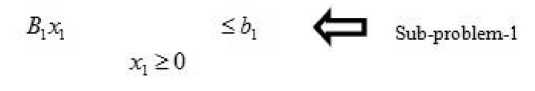
(S_n)   Maximize z = cⁿx_n — Я ^п ( A_nx_n — b )

subject to

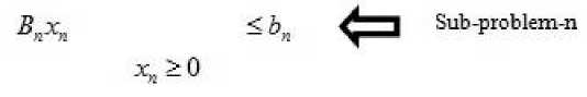
Here Я,Я2,......,% are representing non-negative Lagrange’s multipliers. Here whole problem has decomposed into n sub-problems. Here sub-problems are denoted by S ,S ,......, S respectively.

Step 2: Generation of master problem depends mainly of the corresponding decomposition technique. Here we present master problem obtained for Dantzig-Wolfe decomposition algorithm [5] to demonstrate decomposition procedure for example.

kkk l1l        l2llnl

(M) Maximize z = E9 c Xj + E9c x^ ++ E9c xn i=1                  i=1

subject to

kk    k

»4x / + Е Д А 2 x l + + EAAA <  b

I=1                  I=1                                    I=1

k

E 9 = 1

I=1

k

E 9 = 1

l =1

Ц > 0,i = 1,...., n

Here Ц are representing new variables achieved for master problems and the master problem is denoted by

“M” here.

Step 3: Finally, optimal solution obtained when sum of sub-problem values become equal the master

problem value i . e .

V ( 51) + V ( 52) +.........+ V (Sn) = V (M )

Here V ( S 1 ), V ( S 2 ), problem value.

, V ( S ) are representing sub-problem values and V ( M ) is representing master

2.4. Decomposition Based Pricing (DBP)

This technique was developed by Mamer and McBride [9]. In this section, we have discussed decomposition based pricing algorithm briefly in the following steps.

Step 1: Relax complicating constraints by subtracting from objective function of the original problem. Decompose the whole problem into sub-problems and a master problem. Solve sub-problems and generate master problem by deleting those variables which do not provide non-negative values from the original problem.

Step 2: Stop when sub problem value and master problem value become equal. Otherwise repeat the previous steps.

In the next section, we have discussed about some existing techniques for solving SP problems.

• 3.    Existing Techniques

• 3.1.    L-shaped Method

• 3.2.    Nested Decomposition Technique

There are numerous existing techniques for solving SP problems. In the current section, we have discussed L-shaped decomposition technique, nested decomposition technique and stochastic decomposition technique briefly as follows.

This method was developed by Slyke and Wets [12]. It was developed by using a decomposition technique named Bender’s decomposition [2]. It contains the following steps.

Step 1: It decomposes the whole problem into two stages first. The first stage problem leads to a master problem and the second stage problem leads to a sub-problem.

Step 2: The second stage objective function is approximated by using a piecewise linear convex function. Then approximation is developed iteratively, and convex function is typically represented in a master program using a cutting plane approximation.

One of the drawbacks of this method is that, when the number of scenarios is much too high it is very difficult to solve the problem by using this method [6].

This is a solution procedure of multi-stage SP problems. It just likes a recursive version of L-shaped method. In this procedure, a problem mainly solved sequentially and it can be represented by a scenario tree representation with the change of associated probability with time. We discussed it briefly by the following steps [10].

Step 1: Parent nodes send proposals for solutions to their children nodes.

Step 2: Child nodes send cuts to their parent nodes. There are different “sequence procedures” that tell in which order the problems corresponding to different nodes in the scenario tree are solved.

• 3.3.    Stochastic Decomposition

• 4.    A Multi Period Stochastic Model

  “Agora” is a renowned super shop market in Bangladesh. There are many branches of it in different areas of Dhaka city which is the capital of Bangladesh. Management committee of this market has to collect various types of goods from different locations of Bangladesh and have to make a budget and a plan to maximize profit. They have to make budget with combinations for all goods and other sectors. They have own inventories and transportation facilities. They have to conduct several trips in different times to collect goods. But their profit is not certain all times. It may change due to some uncertain incidents such as political conditions, price of goods, demand of customers etc. To develop this model we have collected data of year 2014. We divide the whole year into four time periods. Each period consists of three months. We have considered “January to March” as period 1, “April to June” as period 2, “July to September” as period 3, and “October to December” as period 4. We have collected data for twelve different products these are rice, wheat, pea, sugar, shrimp, hilsha, squid, banana, chicken, egg, beef and mutton etc. We have considered their transportation costs, packing costs, purchasing costs, personnel costs, holding costs. We have considered three different scenarios of an uncertain situation “political conditions”. This uncertain matter hampers to collect goods, makes transportation problems and lacks of customers safety etc. Our considered scenarios are “good political condition”, “normal political condition”, and “bad political condition”. By good political condition we mean that no political obstacles and proper safety of customers, by normal political condition we mean that no political obstacles but lack of safety of customers suddenly, and by bad political conditions we mean that political obstacles and lack of safety of customers. The cost’s unit is in million (dollar) per hundred ton goods collected and sold.

• 4.1.    Formulation of Multi Period Stochastic model

This technique was developed by Higle and Sen [7]. It consists of the following steps.

Step 1: It operates with an adaptive sample size.

Step 2: Unlike the L-shaped method, which solves a sub-problem for each scenario for each cutting plane constructed, it uses recursive approximation methods based on previously solved problems to bypass the solution of the vast majority of the sub-problems that would otherwise be solved.

In the next section, we have developed a multi period stochastic model. We developed this model by collecting data from different branches of a super shop market located different areas of Dhaka city in Bangladesh by our direct communications.

We do not present details data here due to its volume. If readers are interested then they can contact with authors. In the next section, we present formulation of our model.

Before mathematical formulation of the model discussed in the previous section, we have discussed basic notations that are relevant with our work in this section. We have calculated total cost for transportation, holdings, packing, purchasing, and personnel. Then calculated profit by subtracting total cost from selling price. The parameters, decision variables and formulation have discussed below.

Indices

• •    t , number of time periods.

• •    to , numb er of scenario s.

Uncertain parameters

• •    C T , profit for periods T = 1,..., t and three scenarios where i = 1,..., to .

• •    A T , cost schema for periods T = 1,..., t and three scenarios where i = 1,..., to .

• •    p^T , probability for periods T = 1,..., t and scenarios i = 1,..., to .

Deterministic parameter

• •    Ь , maximum budget for each trip for each scenario and for each month.

Stochastic decision variables

• •   X T , amount of goods collected and sold in period T = 1,..., t for three scenarios where i = 1,..., to .

We have considered three different scenarios i.e. to = 3 and four periods i.e. t = 4 .

Formulation to                     to                      toto

Maximize z = £p1 c1 xT -^p2cixT I ^picixT + Уp4cxT(1

i=1                   i=1                     i=1

subject to to

У A x T ^ ь ii

i=1

to

У A ² x T ^ ь ii

i=1

to

У A ³ x T ^ ь ii

i=1

to

У A ⁴ x T ^ ь ii

i=1

xT > 0, where T = 1,...,t, i = 1,..., to and t = 4, to = 3

In the next section, we have discussed algorithm of our proposed technique. We have explained it on the basis of the formulation of multi period stochastic model.

• 5.    Algorithm of the Proposed Technique

At the first step, we initialize the parameter for number of iterations, and then discuss the selection procedure of Lagrangean multiplier X . After that we have decomposed the whole model into sub-problem and master problem. We have discussed the details procedures in the following steps.

Step 1: k ^ Set number of iterations.

Step 2: Pick an initial set of prices X and this can be chosen by any one of the following alternatives.

• (i)    Start with Я¹ = 0 . Or, start with Я ¹ >  0 as the dual prices from the relaxed constraints of the LP relaxation. Or,

• (ii)    Start with /J > 0 such that Max(CT — $ At) > 0, where T = 1,..., t.

Step 3: Solve the sub-problems,

5 ( x , X^k ): Maximize ^ p T c T x T — X^k (£ A T x^T — b )                                       (16)

i=1                         j =1

subject to to

У A T x T <  ь ii

i=j+1

xT > 0, where T = 1,...,t

Here index j is representing complicating constraints, to is for number of scenarios and t is for number of periods.

Step 4: Master problem will be generated from original problem by deleting those variables which do not have non-negative values. Solve the following restricted master problem.

M ( x , £ ): Maximize T p T C T x T                                                    (17)

i=1

subject to to

T A T x T <  b

i=1

xT e I, where T = 1,...,t

Here I is a non empty set of all variables which give non-negative values in sub problems.

Step 5: For stopping criterion, we use two alternate methods.

• (i)    Stop when the objective value of the sub-problem and the restricted master problem are equal i.e.

• (ii)    Stop when no new variables come into the restricted master. Else go to step-2.

• 5.1.    Computer Code in AMPL

• 5.2.    Period by Period profit Comparisons

• 6. Conclusion

In the current section, we have developed an AMPL code according to our algorithm. This code consists of an (a) AMPL model file, (b) AMPL data file and (c) AMPL run file. Due to the volume we do not present computer code here. But if the readers are interested then they can contact with the corresponding authors.

In this section, we have presented a comparison between profits obtained for different time periods for three different scenarios and presented a discussion. Due to the volume details optimal solution are not presented in this paper. If readers are interested then they can contact with the corresponding authors. Period by period profit comparisons has presented in Fig.1.

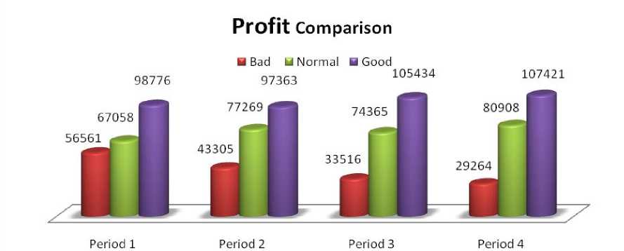
Fig.1. Comparison between Profits

In Fig.1, red, green and blue charts are representing scenarios for bad, normal, and good political condition and the values corresponding to each chart are representing profits for each scenario. For example, the amount $ 98,776 is representing the obtained profit for scenario good political condition in period 1 and similarly for the others. The amount has been calculated in dollar. Naturally political condition is a key factor for a business organization. It has direct impact on its profit or loss. From above figure, we clearly observe that in each period highest profit has made when political condition remains good. We also see that profit has decreased gradually period by period for bad political condition and it’s seem to us that it will be very horrible for the company if profit decreases in such a way. We see from the figure that rate of change of profit is not too high for normal political condition but it’s quite good and if political condition remains like that overall in a year the company has not to make a loss. By analyzing the overall profit, we find that highest profit has made in period 4 that is during the month October to December and it is $10,74271.Finally, we can make a forecast that the company must be cautious for the bad political condition and have to take some plans such as advance collection of commodities which are not raw or increase number of inventories in the conventional locations etc so that they have not to fall in risk in such situations and have not to delay in deliveries ordered by customers. In the next section, we have drawn a conclusion about our work.

In this paper, we presented a new technique for solving multi period SP problems. To develop this technique, we used idea of DBP. We developed a model and analyzed the business policy of super shop markets in Bangladesh. We collected one year data to develop this model. We presented the model with formulations in details and demonstrate its solution procedure by the algorithm of our developed technique. By presenting a comparison between profits, we forecasted that a company such as super shops have to make a multi variable plan to decrease their risk to avoid loss. We are confident that this is the first work with super shop business policy in Bangladesh. We hope that this work will be an example for other such works in future.