A Relook and Renovation over State-of-Art Salt and Pepper Noise Removal Techniques

DIGITAL images play an important role in real life. But different types of noises, uniform, impulsive, gaussian, gamma, rayleigh etc. can severely damage the information in the original image. These noises generally caused by defocusing of camera lenses, scanners or digitizers [18]. Moreover when an image is passed by a channel it also may get contaminated by noise. Over the years different techniques have been evolved to remove various types of noises. Salt and pepper is one of the impulse noises where some pixels get maximum and some get minimum value in the range of (0-255) [23]. Well known traditional filters many times fail to remove this type of image noise as it requires. Special types of linear and non-linear filters have been evolved during last three decades for the purpose of this kind of noise removal [1-17, 19-22, 24-37]. The simplest way for removing salt and pepper noise is by using mean technique which is first applied on image by A. Kundu [5] in 1984. The filter is recognized as MF (Mean Filter), which uses 3×3 windowing for averaging operation. Previously in 1971 SMF (Standard Median Filter) is first median filter introduced by Tukey [12] and successively used by Pratt [34] in image processing in 1975. After that in 1977 SMF is revised by Tukey[13]. Median Filter effectively modified by H. Hwang in 1995 to produce AMF(Adaptive Median Filter) [10]. In the year 1994 Sun and Neuvo [32] introduced switching system and PSMF (Progressive Switching Median Filter)[37] is introduced by Z. Wang using the switching scheme iteratively in the year 1999. Later in 2007 a new decision based filter DBA (Decision Based Algorithm) [17] is introduced by K. S. Srinivasan. In 2010 un-symmetric trimming concept is added by K. Aiswarya to median filter to produce DBUTMF [14] (Decision Based un-symmetric trimmed median filter) and later in 2011 it is modified to MDBUTMF [29] (Modified Decision Based un-symmetric trimmed median filter) by S.Esakkirajan. None of the stated well known filters provide satisfactory result that can be accepted undoubtedly.

Rest of the paper is organized as follows. Next section II presents review of some linear and non-linear filters contemporary to this research. Section III presents the contribution of the recent filters. Section IV presents the scope of improvement of findings over traditional filters.

Section V presents the discussion and analysis. The paper is ended with a section (Section VI) demonstrating the conclusion and future scope of this present work.

II. Review of Some Linear and Non-Linear Filters

A. Mean Filter (MF)

Linear spatial filtering is the first step to smooth the digital image. The process of filtering of a noisy image is given below.

Step 1: A 3 x 3 matrix (S_xy) was created centering the point (x, y).

Step 2: The arithmetic mean was computed taking the intensity value of the pixels of the corrupted image g(x, y) in the defined area S

Step3:             xy.

2) The edges of an image will be distorted.

B. Standard Median Filter (SMF)

One of the most popular and simplest non-linear filters is SMF. Again SMF is called median smoother, mainly based on replacing the value of a pixel by median of the pixels of a 2-D window of size 3×3 taking the regarded pixel in the middle of the window.

Replace I(i, j) = median(k, l) e W

Where Wwas a set of pixels in the window of size (3 × 3) centering the co-ordinate (i, j) and ‘I’ was the output image. The simultaneous process had been followed throughout the noisy image. The entire process has been cleared by the following example.

f ^ˆ (x,y) =

3 x 3

(Zs,teSxyg (s, t))

Input:

Where f (x,y) denoted the value of the said pixel in the restored image then

Example:

Input:

	2	2	4
	7	3	8
	5	1	13

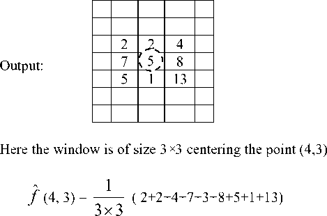
= 5

Advantage:

• 1)    The image is smoothed in a very simple way.

• 2)    It can remove the low level impulse noise.

Disadvantage:

1) It does not consider whether the pixel is corrupted or not, so the uncorrupted pixels are also replaced.

	2	2	4
	7	3	8
	5	1	13

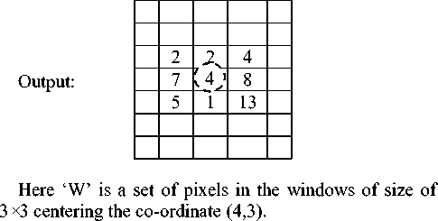
I(4,3) = median {2,2,4,7,3,8,5,1,13}

= median {1,2,2,3,4,5,7,8,13} (The values are sorted in ascending order)

= 4

Advantage:

• 1)    SMF is more effective in real life when the noise percentage is low.

• 2)    Without reducing the sharpness SMF is useful to preserve the edges of an image.

Disadvantage:

1) Its activity is poor when the number of corrupted pixels are greater than the no of uncorrupted pixels in that window.

C. Adaptive Median Filter (AMF)

In Standard median filter the window size was fixed but in AMF the window size was variable i.e. w x w,

starting w=3 and was increased by w=w+2 until the centered pixel was not in between the minimum and maximum intensity value of the pixels in the window or the window size was maximum corresponding to the coordinate (x,y). After setting the window w x w centering the point (x,y) the minimum pixel value (W min ) and maximum pixel value (W max ) in the window were determined. The AMF has two steps.

• 1)    If the centered pixel value is in between W_min and W_max then the pixel will remain unchanged.

• 2)    Otherwise the centered pixel will be replaced by the median of the pixel values in the said window.

Advantage:

• 1)    At most all the respected noisy pixels can be replaced.

• 2)    For variable window size the AMF is effective than SMF when the noise level is high.

Disadvantage:

• 1)    For the border pixels the window size cannot be increased more.

• 2)    Increasing window size leads to blurring.

• 3)    The edges become smeared.

• D.    Progressive Switching Median Filter (PSMF)

The switching system has been adopted in PSMF.

There are two parts in PSMF:

• 1)  Noise Detection

• 2)  Noise Filtering

• 1)  Noise Detection:

Taking the values after every iteration two image sequences one grayscale image sequence and other binary flag image sequence were generated.

In binary flag image ‘0’ and ‘1’ represented whether the pixel was good or an impulse respectively. Firstly all pixels were considered as good one. A w x w matrix (w is an odd integer not less than 3) was generated taking the corresponding pixel (X) at the center. Then the median (m_d) of the pixels in the said matrix was find out and a pre-defined threshold(T_d) value was taken.

if (abs(xi - md)

else the pixel  considered  as  impulse  and  the corresponding binary flag = 1.

This process is continued to nth iteration. After nth iteration the generated binary flag image was used for noise filtering.

• 2)    Noise Filtering:

The previous binary flag image was taken on account.

Then two image sequences one grayscale image sequence and other binary flag image sequence were generated.

In the binary flag image ‘1’ represents corrupted and ‘0’ represents uncorrupted .Taking corresponding corrupted pixel at center a w x w matrix was considered in the grayscale image where w is an odd integer not less than 3. The corresponding center pixel was replaced by the median of the uncorrupted pixels in the said matrix simultaneously the corresponding pixel of the binary flag image was replaced by ‘0’.

If the number of uncorrupted pixels was even then the median was calculated by the arithmetic mean of left and right median.

Once a corrupted pixel was replaced, it was considered as an uncorrupted pixel in the next iteration.

Proceeding in this way after nth iteration there would be no corrupted pixel which had not been replaced.

Advantage:

It restored the image with minimizing the blurring effect that occurs in AMF at low noise density.

Disadvantage:

When the noise level is high the image may not be recovered satisfactorily.

• E.    Decision Based Algorithm (DBA)

DBA basically came through the concept of SMF. In SMF each pixel was replaced by the median of its neighbourhood pixels inside the selected kernel. But in DBA all the pixels were not replaced as in this process the pixels were firstly checked whether it was corrupted or not. After detection if the pixel was detected corrupted, it was replaced.

• 3)    Noise Detection:

• a)    A 3 x 3 kernel was selected considering the processed pixel in the center.

• b)    The pixels in the said kernel were sorted first row wise then column wise in ascending order.

• c)    The first element of the window was minimum, the last was maximum and the middle was median valued.

• d)    If the corresponding pixel was in between the minimum and maximum value then the pixel was considered as an uncorrupted pixel otherwise it was corrupted. If it was uncorrupted it was left unchanged.

• 4)    Noise Removal

If the corresponding pixel was corrupted then it was replaced by two ways.

• a)    If the median value was in between the minimum and maximum value then the corrupted pixel was replaced by the median.

• b)    If the median was either minimum or maximum i.e. ‘0’ or ‘255’ then the corresponding pixel was replaced by its neighbourhood uncorrupted pixel.

Advantage:

Here the edges are recovered better.

Disadvantage:

Repeated replacement of neighbourhood pixels produces streaking effect.

• F.    Decision based un-symmetric Trimmed Median filter (DBUTMF)

The DBUTMF was the developed process of decision based algorithm (DBA) which more or less as DBA.

• 1)    Here first a 3 x 3 matrix was created taking the corresponding pixel as center of the matrix. If the intensity value of the corresponding pixel lied between ‘0’ and ‘255’ then the pixel remained unchanged.

• 2)  Again if the corresponding pixel was a corrupted

one then all the intensity values of the pixels of the 3 x 3 matrix were stored at an array and observed whether the starting pixel and the ending pixel was ‘0’and ‘255’ respectively. If the left and right extreme value of the stored array was ‘0’ and ‘255’ respectively then the corrupted pixel was replaced by the median of the pixels in the 3 x 3 matrix excepting the corrupted pixels in the said window.

Advantage:

It gives better result up to noise level 70%.

Disadvantage:

If all the pixels of the selected window are corrupted then trimmed median value cannot be obtained.

• G.  Modified Decision based un-symmetric Trimmed

Median filter (MDBUTMF)

In MDBUTMF the corrupted image was checked pixel wise and the process stated below had been adopted.

• 1)    At first the corrupted pixels were identified i.e. ‘0’ and ‘255’.

• 2)  2-D window of size 3 x 3 was created taking the

corresponding pixel as a center one.

• 3)    If the intensity value of the centered pixel was in between 0 and 255 then the pixel remained unchanged.

• 4)    Again if the intensity value of the centered pixel was ‘0’ or ‘255’ and all the pixels in the selected window are not ‘0’ or  ‘255’  then the

corresponding pixel was replaced by the median of the intensity values of the pixels in the said window excepting ‘0’ and ‘255’.

• 5)    Moreover, if the intensity value of the centered pixel was ‘0’ or ‘255’ and all the pixels in the selected window were ‘0’ or ‘255’ then the corresponding pixel was replaced by the mean of the intensity values of the pixels in the said window.

Advantage:

If all the pixels of the selected window are corrupted, then also the desired value can be obtained by mean.

Disadvantage

This process could not perform better at noise density 80%-90%.

• III.    Contribution Of The Recent Filters

Table 1. Recent Contributions

Sl. No	Papers	Contributions
1	[36]	A new filter is proposed comprises of non-local mean filter and adaptive median filter. In detection phase the noisy pixels are detected using adaptive median filter. The noisy pixels are replaced using non-local mean filtering technique.
2	[4]	A new filter for local edge preservation is proposed. 16 different sets are formed by gradient calculation. For each noisy pixel the window type is decided upon the neighbourhood pixels. Then for each set of window four gradients are estimated based on corrupted pixels and estimated un-corrupted pixels. Lastly the center corrupted pixel is replaced by the minimum of the four gradient values.
3	[21]	Adaptive window size is determined by continuously enlarging the window size until the maximum and minimum values of two successive windows are equal respectively. Then the center pixel is regarded as the noisy pixel if it is equal to minimum or maximium value. Then the noise candidate is replaced by the weighted mean of the corresponding window.
4	[22]	A histogram weighted mean filter is proposed. A 5×5 sliding window is taken as a kernel. Noisy pixels are replaced by the histogram function weighted mean filter.
5	[2]	A joint scheme of wavelet transformation using iterative noise density and median filtering is proposed. Firstly the wavelet transform decomposes the noisy image in form of approximate and detailed components. Then median filtering is applied on the approximated coefficients of wavelet transformations and the noise variance is estimated. At the end inverse transform is done for getting the de-noised image.
6	[28]	A new row-coloumn based operation is introduced. Here intensity values of a greyscale image ranging from 0-4 and 251-255 are considered as noise. The proposed method approximated the value of the noisy pixel using neighbourhood pixels along the rows, columns and both together in multi-stage conditional and unconditional operations.

• IV.    Scope Of Improvement Of Findings

Initially it has been stated only the filters and their advantages and disadvantages. In this section, a few observations of different filters were detected and has been tried to provide some solutions for the scope of improvement.

Modified Mean Filter (MMF)

Two minor changes in the mean filter are proposed here.

• 1)    The size of the matrix will be greater when the noise level is high.

• 2)    Detecting whether the centered pixel is corrupted or not. If the center pixel is corrupted, then only it should be replaced. Again at the time of arithmetic mean the corrupted pixels in the created matrix must not be counted. If f (x,y) denote the said pixel in the input image and f (x,y) denote the said pixel in the restored image then

• 3)

x f ^ˆ (x,y) = ^{∑ i i}

n

Where x denote the intensity values of the uncorrupted pixels in the matrix and n denotes the number of uncorrupted pixels in the same matrix. Here we want to say that only the corrupted pixels would be changed and this modified mean filter can give a better result even at high noise levels. According to the findings the comparison between the existing and MMF in respect of PSNR is shown in Table 4. of section V.

Modified Adaptive Median Filter (MAMF)

The disadvantage of SMF has been more or less removed by AMF but here also total disadvantages cannot be overcome. A few minor changes are introduced in the proposed MAMF.

Noise Detection:

As the input image is a salt and pepper noisy image so the intensity value of the corrupted pixels will be ‘0’ or ‘255’. So, a pixel is corrupted or not and whether it should be replaced or not need not be examined by creating a matrix centering the said pixel.

Noise Removal:

• 1)    The corrupted pixel at the border can be replaced by making a matrix taking the corrupted pixels at any corner and the corrupted pixels can be restored by the median of the pixels in the matrix.

• 2)    The size of the matrix depends on the percentage of noise as shown in Table 2.

• 3)    A sorted array must be formed taking the values of the uncorrupted pixels from the created matrix.

• 4)    The corrupted pixels can be replaced by the median of the said array by which the blurring and the smearing of the edge issues can be solved. According to the findings the comparison of the

existing filters and the proposed in respect of PSNR is shown in Table 5. of section V.

Table 2. Variation Of Window Size With Respect To Noise Percentage

Noise Percentage (p)	w max ×w max
p < 25%	3×3
25% < p < 50%	5×5
50% < p < 70%	7×7
70% < p < 90%	9×9

Adaptive Decision Based Algorithm (ADBA) :

As before DBA tried to overcome the disadvantage of PSMF. But when the created matrix is only comprised of corrupted pixels, the method of replacement of the pixel is made by the mean of four neighbourhood pixels which caused streaking effect.

Keeping this problem in mind a few minor changes are introduced in the proposed ADBA. To overcome the drawback the matrix size should be increased and the replacement can be made only by the mean of the uncorrupted pixels.

According to the findings the comparison of the existing filters and the proposed in respect of PSNR is shown in Table 6. of section V.

Conditionally Modified Decision based un-symmetric Trimmed Median filter (CMDBUTMF):

The DBUTMF and MDBUTMF are more or less same excepting the position when the 2-D selected window 3×3 is full of corrupted pixels. MDBUTMF stated that if the intensity values of all the pixels of the selected window are corrupted then replace the center pixel by the mean of the elements of the window. Here also a pixel is replaced with the help of corrupted pixels and when the noise level is above 80% most of the cases all the pixels in 3×3 window will be corrupted. If the corrupted pixel is replaced by the mean of a few corrupted pixels then the appropriate desired value cannot be obtained.

A few minor changes are introduced in the proposed CMDBUTMF.

If all the pixels in the created matrix are corrupted then the window size can be increased for a certain period (i.e. from 3 to 9 taking the odd numbers shown in Table 2.) and the centered corrupted pixel will replaced by the mean of uncorrupted pixels from the respected window. According to the findings the comparison between the existing and proposed in respect of PSNR is shown in Table 7. of section V.

The well known above said filters has a great contribution over image restoration. If these processes have not been adopted in the image restoration then we would be in dark about the system. So we are bound to be grateful to the existing process.

Basically here the traditional filters are reviewed and analyzed. There were a lots of modern filters introduced, but most of them have used these traditional filters as their base. Here in this paper these new filters also has been analyzed .It has also been explained how the traditional filters made the way for the new filters.

• V.    Disscussion And Analysis

Algorithmically the traditional mean filters and median filters are less complex i.e. they were having low complexity as because the formulation was very easy to implement and the time taken for execution was also small. The adaptive median (AMF) filter follows near about the same formulation but as the window size increased the time taken for execution also greater than the traditional median or mean filters. Then in Progressive Switching Median Filter (PSMF) the formulation becomes more complex and due to the no of iterations the execution time also increased leads to a huge complexity. After that DBA is introduced where window size was small but large time taken for execution because of the row wise, coloumn wise and diagonal wise sorting. Hence the time complexity is also high. Then MDBUTMF was introduced where also the window size was taken small as 3×3 and formulation used the concept of basic median and mean concepts in different conditions so the execution was easy and fast. Hence the complexity is also less.

Quantitative performances of the de-noising techniques are measured by Mean Square Error (MSE), Peak Signal-to-Noise Ratio (PSNR) as defined in eq. (1) and (2) respectively.

MSE=

s

M , N

i

I ( m , n ) - 1 ( m , n ) I

M x N

MSE is the mean square error between original image (j ) and de-noised image (^ | ). M and N are the number of rows and columns in the input image, respectively.

PSNR = 10 log!₀ (255 2 / MSE )         (2)

Table 3. presents the PSNR values from eq. (1) and (2) of the well known traditional filters for comparison with respect to the Lena image in the noise range 10%-90%.

Table 3. Psnr Values Of Different Filters For Lena Image At Different Noise Densities

Nois e in %	PSNR in dB
	SMF	AMF	PSMF	DBA	DBUTM F	MDB UTMF
10%	26.34	28.43	30.22	36.40	36.51	37.91
20%	25.66	27.40	28.39	32.90	33.42	34.78
30%	21.86	26.11	25.52	30.15	31.25	32.29
40%	18.21	24.40	22.49	28.49	29.51	30.32
50%	15.42	23.40	19.13	26.42	27.08	28.18
60%	11.13	21.00	12.12	24.83	25.52	26.40
70%	9.93	15.30	9.84	22.61	23.41	24.30
80%	8.70	10.30	8.10	20.32	20.93	21.70
90%	6.60	7.93	6.57	17.14	17.92	18.40

Fig.1. presents the graphical representation of the PSNR values for the same Lena image at 70% noise density but for visual representation and easy comparison.

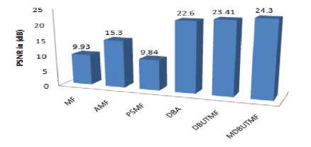
Fig.1. PSNR values of different traditional filters at noise density 70% for Lena Image

Fig.1. shows the gradual increasing PSNR values graphically for the traditional filters. Only in case of Progressive Switching Median Filter (PSMF) the value decreases. As the graph shows the PSNR values at 70% noise density the PSMF could not perform well because the filter works well only at lower noise density. From Table 3. and Fig.2. it is affirmed that as the PSNR increases the visual quality of the images improves and decrement of PSNR distorts the image quality. Now from the equation (1) and (2) it can be stated that increment of PSNR results in decrement of MSE value and vice versa. So it can be said that PSNR is inversely proportional to MSE.

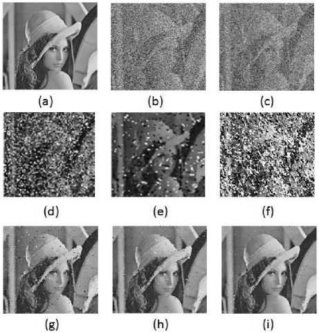
Fig.2. Result of different filters on Lena image (a) Original Image (b) 70% noise corrupted image (c) MF (d) SMF (e) AMF (f) PSMF (g) DBA (h) DBUTMF (i) MDBUTMF

Table 4. Comparison of Psnr Values for Lena Image At 70% Noise Density

Noise in %	PSNR in dB
	MF	MMF
70%	14.62	24.51

Table 5. Comparison of PSNR Values for Lena Image At 70% Noise Density

Noise in %	PSNR in Db
	SMF	AMF	MAMF
70%	9.93	15.30	24.21

Table 6. Comparison of PSNR Values for Lena Image at 70% Noise Density

Noise in %	PSNR in dB
	PSMF	AMF	ADBA
70%	9.84	22.61	24.84

Fig.5. MSE values of different traditional filters at noise density 70% for Lena Image

Table 7. Comparison of PSNR Values for Lena Image at 70% Noise Density

Noise	PSNR in dB
in %	DBUTMF   MDBUTMF	CMDBUTMF
70%	23.41           24.30	27.48

Fig.3. represents the visual result of the new filters discussed in the contribution at 70% noise density with respect to Lena image.

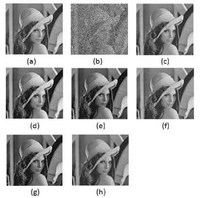
Fig.3. Result of different filters on Lena image (a) Original Image (b) 70% noise corrupted image (c) [36] (d) [4] (e) [21] (f) [22] (g) [2] (h) [28].

Fig.4. shows the PSNR values graphically for the recent filters. These new filters works fine at noise density 70%.

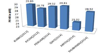
Fig.4. PSNR values of different traditional filters at noise density 70% for Lena Image

Fig.5. shows the MSE values graphically for the recent filters. These new filters gives lower mean square errors at noise density 70% that shows the efficiency of these new filters over the traditional well known filters.

• VI.    Conclusions

Traditional and state-of-the-art filters for salt and pepper noise removal have been taken in to an account in this work. Among these filters, MF, SMF, AMF, PSMF, DBA, DBUTMF and MDBUTMF are specially explored and their comparative performances have been presented with an emphasis of applications at high noise density levels. Contributions of the papers in this domain are looked backed, renovated and presented in a more comprehensive way by which the work may be appropriate for any individuals with general science background. The main focus of investigations reported in this paper is about the well known filters; simultaneously the updated recent filters are also stated. It has been observed that the performance of the above filters was not satisfactory where the noise level is particularly high. This technology gap may be targeted to bridge by introducing some modified filters of the above filters.