A Review on Image Reconstruction Using Compressed Sensing Algorithms: OMP, CoSaMP and NIHT

The pioneering works of Kotelnikov, Nyquist, Shannon and Whittaker on sampling of continuous time bandlimited signals [1, 2, 3] showed that signals, images, videos, and other data can be exactly recovered from a set of uniformly spaced samples taken at the Nyquist rate. Due to the high rate of success in digitization, the data generated by sensing systems have also grown huge in size for various applications. Hence, too many samples are produced if the Nyquist criteria is followed. Despite advances in signal processing at higher speeds and storage abilities, this posed a challenge to the computational world.

To address this challenge, compression techniques were adopted, which aims to find the most concise representation of a signal with acceptable distortion. The most popular signal compression techniques which include transform coding are, JPEG, JPEG2000, MPEG, and MP3 standards. In these techniques, the entire signal is acquired and then removal of redundant data is applied in subsequent steps.

The traditional method of acquiring entire signal and then compressing was questioned by Donoho [4] and laid the foundation for a field of Compressed Sensing. Compressed Sensing (CS), or Compressed Sampling, refers to reconstructing signals efficiently from a set of a few non-linear measurements having some incoherent properties [4, 5, 6]. As most of real life signals are compressible in nature and can be represented as sparse signals in some transform domain. As sparse signals having very few non zero coefficients, it can be represented by some linear measurements. Non-linear optimization can then enable recovery of such signals from very few measurements. Hence, CS enables a potentially large reduction in the sampling and computation costs for sensing signals which are having sparse or compressible representation.

In 1795, Prony proposed an algorithm for the estimation of the parameters associated with a small number of complex exponentials sampled in the presence of noise [7]. Around 1900, Caratheodory showed that a positive linear combination of any k sinusoids is uniquely determined by its value at t = 0 and at any other 2k points in time [7]. This corresponds to far fewer number of Nyquist rate samples when k is small. In the early 2000, Blu, Marziliano, and Vetterli developed sampling methods for certain classes of parametric signals which are governed by only k parameters, showing that these signals can be sampled and recovered from just 2k samples [8]. Beurling proposed a method to reconstruct signals from partial observation of its Fourier transform [9]. This approach suggests to find the signal with smallest l1 norm among all signals agreeing with the acquired Fourier measurements bears a remarkable resemblance to few algorithms used in CS.

In this paper, few greedy CS algorithms like Orthogonal Matching Pursuit (OMP), Compressive Sampling Matching Pursuit (CoSaMP) and Normalized Iterative Hard Thresholding (NIHT) are reviewed and their performance is evaluated based on various image quality parameters.

This paper is divided into different sections, where Section II explains the problem formulation of image reconstruction, Section III provides an overview of the reconstruction algorithms and covers Orthogonal Matching Pursuit (OMP), Compressive Sampling Matching Pursuit (CoSaMP) and Normalized Iterative Hard Thresholding (NIHT) algorithm's theoretical aspects and implementation structure. In Section IV, simulation results of these algorithms are presented. Conclusions are presented in Section V.

• II.    Problem Formulation of Image Reconstruction

As per CS theory, an unknown sparse signal, in which the number of nonzero components are far less than its length, can be reconstructed from under determined nonadaptive linear measurements that fulfill incoherence properties. These under determined nonadaptive linear measurement being less than the length of sparse signal, where the linear measurement is independent of the sparse signal. This compressed sensing or compressive sampling model is represented as follows,

• У - ФХ (1) sparse

Where, X_sparse e Rn ^{x 1} is a sparse signal with the number of nonzero components k far less than its length n . Hence, out of n components of signal X only k nonzero components are taken in X_se . Ф e R^{m x n} is a measurement matrix with its number of rows m being less than columns n . Measurement matrix is often called measurement dictionary with each column called atom of the dictionary. Y e R^{m x1} is refereed as measurement signal. Equ. (1) has an infinite number of solutions as it is under determined linear equation. One simple solution can be achieved through Moore Penrose Pseudo inverse method, in its closed form as Ф ^f Y , which is based on the least square criterion. Ф ^f is Moor-Penrose Pseudo inverse of Ф .

For X signal, solution leads to the following sparse , optimization problem,

• , min . x1|WL ^t ■ ^Y = ^Ф Sparse        (²)

X sparse ^e R

Where, . is pseudo norm which counts the number of nonzero components in the input vector. Equ. (2) has

, f n )        ,       „       , .

total I I number of combinations possible, where m is

I ^m )

the length of the measurement signal. Hence, solution of Equ. (2) is an NP-HARD problem. Various Greedy algorithms aims to solve the l minimization problem approximately. l problem could be related to l (0 < P < 1) or even lx problem under some conditions. l and l problem can be represented as follows, x minnxi lIXsparsellp s.t. Y = ФXsparse          (3)

X sparse e R x minnxilIXsparselI    s• t• Y = ФXsparse         (4)

X sparse ^{e R}

Where, . and . represents p-norm and 1-norm of the input vector respectively.

Comparatively, l problem is easier to solve as it is a convex type, i.e. , there exists a unique global solution [11] and can be solved using Basis pursuit (BP) algorithm. The equivalence of l problem with l or l problem requires restrictions on measurement dictionary and the sparsity of the original sparse signal. For measurement dictionary, if the following inequality holds true for any sparse signal X_sparse [11].

Vl— ^ 7 || X sparse | L ^ |Ф X sparse | L ^ V^+ ^ T ( ^ sparse | L (5)

The measurement dictionary is said to be with k ^th order Restricted Isometry Condition (RIC) ^ . For l_v minimization problem stated by Equ. (4), if 2 k ^th order RIC of measurement dictionary satisfies, the solution of l and l minimization problem becomes identical. A more fundamental concern is whether the solution of l problem is equal to the original/sparse signal or not? In terms of RIC, it can be said that when the solutions to Equ. (2) is exactly the original/sparse signal [11].

Another important parameter is called coherence and cumulative coherence of measurement dictionary. The coherence а ( Ф ) and k th order cumulative coherence ^ ( Ф ) of measurement dictionary Ф are defined as [12],

^(Ф) = max|< фi,фj >|

^ i ^(ф) = mmax max i ^E< ^ф , ^ф >1

Where, ф e R m ^x1and ф e R ^{x 1} represents i th (1 <  i <  m) and j ^th (1 <  j <  n) columns of measurement

dictionary. Here I is

set of indices. If

^(ф)<

2 k - 1

or

» - (^k D + A ^(k) <  1 , solution of l ₀ problem and l_x problem becomes identical. So, the Basis Pursuit and the OMP algorithms can be used to recover the sparse signal in compressed sensing [12].

III. Compressed Sensing Algorithms for Image Reconstruction

From above introductory discussion, it can be seen that RIC or coherence represents quality of the measurement dictionary and suggested to have small value [11]. The measurement dictionary is a redundant, which means that the number of columns are larger than that of rows, hence, RIC could never become zero. Similarly, the smallest value of coherence and cumulative coherence of measurement dictionary is favored in CS [12]. In the extreme case, when both of coherence and cumulative coherence become zero, measurement dictionary becomes an orthogonal matrix and sparse signal recovery becomes easier.

As measurement dictionary is redundant in nature, one could never expect that coherence becomes zero. There exists a lower bound of coherence ( ^ ,) , called welch bound . For a real redundant dictionary with size m x n and n <  0.5 m (m - 1), welch bound is given as,

^W = , № (8) у m (n-1)

The Welch bound is ideal condition, which cannot be achieved always by any pair of m and n. Welch bound suggests that, how one could reduce the coherence of measurement dictionary [13] and design measurement dictionary with small coherence value based on alternating projection method. From simulation shown in [13], it is observed that for dictionary with certain dimensions, the coherence could achieve welch bound. Quality of the measurement dictionary can be evaluated from RIC, but here calculation of its k ^th order RIC is impractical as it involves computation of an eigen value of the Gram matrix formed by any k columns. Following equation represents the condition for k ^th order RIC,

5k = max {A„ (ФT, Фi)-1,1 - Amin (ФTФi)} (9)

Where, Ф, is matrix composed of atoms of Ф with index in the set I , A nax (^{Ф T Ф} I ) and A min (^Ф T ^Ф i ) ^are maximal and minimal eigen value respectively. Relationship between RIC and cumulative coherence can be represented by following equation,

бк < Ц1 (k-1)                 (10)

Equ. (10) represents the relationship between k ^th order RIC and ( k - 1) ^th order cumulative coherence. As computation of cumulative coherence is practically possible, one can aim to design dictionaries that ultimately satisfies minimum RIC value criteria. Hence, it is quite reasonable to accept minimum coherence as a criterion instead of RIC to design the measurement dictionary.

In this paper, three different algorithms named Orthogonal Matching Pursuit (OMP), Compressive Sampling Matching Pursuit (CoSaMP) and Normalized Iterative Hard Thresholding (NIHT) are reviewed. These algorithms are utilized for image reconstruction application and their outcomes are evaluated based on various absolute performance parameters.

A. Image reconstruction using Orthogonal Matching Pursuit (OMP) algorithm

An sparse signal with k sparsity value represented as,

(11) sparse           in

Where, X    is sparse signal having only few k nonzero terms. T is sensing dictionary. In other words,

X^ (i) * 0, i O I             (12)

The index set I corresponding to the nonzero components of sparse signal. Sparsity k means that 1 1 | = k , only index values of k sparse signals are considered and remaining set to zero. The basic CS problem can be expressed as

Y = ФX   = Уф X       (13)

sparse           i sparse iOI

Where, Y represents the measurement signal, Ф represents the measurement dictionary and ф e R m ^x1 is the i ^th column or atom of measurement dictionary. As per above Equ. (13), the measurement signal Y is a linear combination of k atoms of measurement dictionary. These atoms and combination coefficients can be determined by nonzero components of sparse signal X . After every iteration, the OMP algorithm selects the atom of measurement dictionary Ф , which is most correlated with the correct residual r . The index of this atom is added into the set of selected atoms ( I ). The algorithm updates the nonzero coefficients of sparse signal using least square technique. Then after, the residual signal is updated using the coefficient and index set is estimated again. After selection of one atom and addition of its index set I , residual is updated as follows,

Let P and P1 defined as the orthogonal projection operator on the column space Ф, and its complement

Is respectively,

P =ФIs =Ф Is f

P1= 1 -P = I-Ф, Ф,f

Is               Is                 IsI

Where ФI$f = (фT ФI$) ФT is the Moore penrose pseudo inverse of Ф . Now, residual signal is redefined Is as, r = Y -Ф, Xsparse(16)

Г = Y-ФФf Y  (•."Xsparse =Фf Y)(17)

r = (I - P)Y(18)

Г = P1 Y(19)

So, orthonormal signal becomes the orthogonal complementary projection on the subspace spanned by all the selected atoms whose index lies in the set I . As per orthogonal complementary projection property, residual r is orthogonal to the selected atoms. Which can be expressed as below,

Ф r = 0   iHIs(20)

In the atom identification process, the identification vector h can be written as, h = ФТ r(21)

The above equation can be rearranged as, hIs =ФV = 0,Is и

Where hI is components of vector h whose index belongs to the index set I and 0 is zero vector with size I s I ■ 1 .

As per Equ. (22), initially only single atom is selected and its index number is added to the index set I . The inner product of this atom with the residual signal becomes null, hence the selected atom could not be reselected again. After k iterations, all the atoms whose index set I are selected and their estimated coefficients are given as,

-Xsparse =(ФT ФI )-1 ФT Y(23)

Xsparse = (ФT ФI )-1 ФT ФI Xsparse   f' Y = ФI ^sparse )

XSparse = Xsparse

As per Equ. (25), If all atoms correctly selected, the reconstructed sparse signal matches with the original one.

For the success of the OMP algorithm, some conditions need to be fulfilled. The first condition is to find the value of RIC that guarantee the success of the OMP algorithm? The answer was given by Mo and Shen [16], if the RIC P ₊₁ of measurement dictionary Ф satisfies,

5 k + 1 = 1/7 k + 1               (26)

Then for k sparse signal, the OMP will recover X from Y = ФX___ in k iterations. A sufficient condition sparse for reconstruction is to recover the sparse signal from under determined linear measurement [12].

Y = Ф X sparse s.t . max\ Ф^f Ф , |< 1        (27)

i 6I C

Which means maximization occurs over all atoms Ф_г, which do not participate in the k sparse representation. Another sufficient condition given for Equ. (27) based on the cumulative coherence of measurement dictionary [12]. The exact recovery condition mentioned by Equ. (27) whenever,

_A ( k - 1 ) + Ц 1 ( k ) < 1           (28)

Therefore the OMP algorithm is successful for k sparse signal recovery whenever Equ.(28) holds true.

As discussed both Equ. (27) and Equ. (28) represents sufficient conditions for the algorithm. Equ. (27) demands for the required index set I of correct atoms, which is unknown beforehand, hence it cannot applied practically. On the other hand Equ. (28) involves only cumulative coherence which is independent of the sparse signal. Hence, based on measurement dictionary or on cumulative coherence, one could evaluate the OMP algorithm for recovery of k sparse signal.

The quality measuring parameters of the measurement dictionary, mutual coherence and RIC are related to each other as follows,

5 k <  ^ 1 ( k - 1 )                   (29)

For over complete measurement dictionary, it's better to calculate cumulative coherence as compare to RIC. Instead of designing measurement dictionary with small

RIC, which is impractical, one can attempt to design with small coherence value as mentioned [23, 24].

Incorporation of Sensing dictionaryFigures and Tables

Let matrix ^oRmxn be sensing dictionary of the size m× n. If input data or signal is not sparse in direct form, it can be sparsified using a sensing dictionary, i= max ψT r                 (30)

1 ≤ j ≤ n    ^j

Where, ψ ∈ R^{m × 1} is j ^th atom of sensing dictionary Ψ and r is residual. As, RIC for measurement dictionaries, a similar value termed generalized RIC is defined [15]. For a pair of measurement and sensing dictionaries the following inequality for k sparse signal X is,

( ^{1 - δ} k ^' ) ^X sparse 2 ^{≤ Ψ T Φ X} sparse   ^≤ ( ^{1 + δ} k ^' ) ^X sparse 2 (31)

The parameter δ ^' is termed as k^th order generalized RIC. As, RIC of measurement dictionary, there is a relationship between the eigenvalue of type Gram matrix ψ^T φ ? and generalized RIC for any index set I satisfying

I ≤ k , then exists the following inequality.

( 1 - δ k ^' ) ≤ λ min ( ψ I^T φ I ) ≤ λ max ( ψ I^T φ I ) ≤ ( 1 + δ k ^' )   (32)

Where, λ _min ( ψ _I ^T φ _I ) and λ _max ( ψ _I ^T φ _I ) are minimal and maximal eigen value of type Gram matrix ( ψ ^T φ ) respectively.

From Equ.(32), the calculation of generalized RIC seems to be computational difficult as the eigen value of total nm number of Gram matrix is required to be calculated.

The identity vector is given as, h =ψrT                 (33)

Let’s discuss a sufficient condition, based on which the OMP algorithm involving sensing dictionary succeeds in recovering k sparse signal in CS. Suppose that (k+1)^th order generalized RIC of sensing measurement Ψ satisfy the following inequality,

δ ^'  <   ¹                       (34)

k + 1       _{k + 1}

Then for any k sparse signal X , the OMP will recover X    from Y=ΦXin k iterations [14]. The sparse                        sparse

OMP algorithm could select the correct atom in the first iteration and after it, if is replaced by residual r , OMP could select next correct atom and so on.

Now let’s define mutual coherence and cumulative coherence for sensing and measurement dictionary. Let

ψ and Φ are sensing and measurement dictionaries respectively. Mutual coherence and cumulative mutual coherence are defined as,

µ' = max ψiT φj(35)

1 ≤ 1 _j ≤ n

µ' =max max ∑ψTφ(36)

1     Is =k 1≤i, j≤n,i∉IS, j∈IS     ISi j

Where, ψ ∈ R^{m ×1} = i^th atom of sensing dictionary Ψ and φ ∈ R^{n × 1} = j^th atom of measurement dictionary Φ .

In the OMP algorithm, when sensing dictionary Ψ is involved, right atom will always be selected if,

(ΦTICΨI)-1ΦTIΨIC≤1(37)

Which always satisfied if,

µ'(k) +µ'(k-1) < β(38)

Where, β = minψT φ . 1≤i≤n

Compare to Equ. (37), sufficient condition given by Equ. (38) can be easily determined by the cumulative mutual coherence of sensing and measurement dictionaries. From Equ. (38), one can observe that mutual coherence should be minimized by designing sensing dictionary with respect to the measurement dictionary. Minimization of cumulative mutual coherence also makes sense for generalized RIC, because relationship exists between generalized RIC and cumulative mutual coherence. ( k-1)^th order cumulative mutual coherence and k^th order generalized RIC of sensing and measurement dictionaries have the following inequality [15].

δ k ^' ≤ µ 1^' ( k - 1 )                    (39)

Above statement suggests that minimization of ( k-1)^th order cumulative mutual coherence would bound the value of k^th order generalized RIC. Generalized RIC with small value is preferable in the OMP algorithm. There exists a relationship between mutual coherence and cumulative mutual coherence which is,

µ ₁ ^' ( k ) ≤ k µ ^'                     (40)

Based on the above equation, design a sensing dictionary with respect to the given measurement dictionary with small mutual coherence to force the cumulative mutual coherence to be small. The steps involved in the OMP are explained in Algorithm 1[17].

Algorithm 1: Orthogonal Matching Pursuit (OMP)

• •    Input image X

• •    Sensing Dictionary Ψ of dimension m × n to produce sparse signal from input signal X =Ψ X sparse           in

• •     Sparsity level k

• •    A measurement matrix Φ of dimension m × n

• •    A data vector of dimension m

Output

• •    An estimate X sparse of dimension n of the vector

X sparse .

• •    The support I ∈ R^k of X sparse

• •    New approximation of y of data vector y

• •    m dimensional residual r = y - y

Procedure

• I) . Sparsification of Input Signa l

• •      Initially take entire input signal or image as

input X _in

• •     As input is not sparse in direct form, it can be

sparsified using sensing dictionary, which is over complete DCT basis. The over completeness of this dictionary depends on various parameters, as discussed in theory.

• •      After finalizing the sensing dictionary,

determines the sparsity level k applied to signal input X _in .

• •     Now take the residual r

• •      Initialize with r = X , find the identity vector

using, h =ΨT (projection vector). After applying identity vector  h,  calculate the maximum value of its projection, and update the index of sensing dictionary.

• •     After taking maximum term and its index I ,

repeat the same for k levels of sparsity and update the index accordingly. Now α =Ψ^-1 X , Where α = atoms of dictionary having nonzero value.

• •     Then after update residual, Apply

r = X - Ψ α formula for residual update. Hence, after atom by atom updation, final identification vector having only k non zero values and can be obtained.

• II) . Initialize

• •      Initially, size of measurement matrix Φ is

calculated by m = C log ( n / δ ) , Where n = number of dictionary atoms, C =constant and δ = RIC

• •     Then after calculate, Y =Φ X

,                sparse

• III) . Identity

• •     Project the residual onto the measurement

dictionary Φ to identify the columns (i.e., atoms of the dictionary) that help in estimation, which takes total k iterations to produce k index values.

• •      In Identification process, projection initialize with

r = Y, h = ΦTr and this Equ. can be rearranged as h =ΦT T r . Where h are components of vector h whose index value belongs to the index set I . After completion of first iteration, update the index set to nonzero as well as zero coordinates. Now, ^       ^^

X sparse =Φ ^T _I Y then Y =Φ _I X sparse . Update

^

r = Y - Y and utilize it for the next iteration and repeat above procedure. Finally reconstructed signal is reproduced by putting non zero and all zero values together.

^

• •      X sparse can be utilize to obtain reconstructed signal

^

^{as, X} reconstructed ^{= Ψ X sparse .}

• •      Reconstructed X_{reconstructed} signal is compared with

input signal X and performance is analyzed.

The OMP algorithm can recover sparse signals with high probability using random measurement vectors that are independent of signals, but it cannot provide guarantees for recovery of all sparse vectors [17, 28]. It is highly efficient in the reconstruction of high sparsity vectors, but costly in case of non-sparse vectors. But, due to simplified implementation, the OMP algorithm is an attractive alternative to convex relaxation algorithms.

• B.    Image reconstruction using Compressive Sampling Matching Pursuit (CoSaMP) algorithm

The other greedy algorithm, Compressive Sampling Matching Pursuit (CoSaMP) is a modified OMP algorithm, which incorporates features that guarantee comparatively better performance.     Theorem A guarantees its performance on noisy samples and shows that that run time is nearly proportional to the length of most of the vectors [18].

For a k -sparse signal X collected in the form

Y =Φ X , a vector v can easily form the proxy of the signal v    , which approximates the energy.

Particularly the k -largest components in v corresponds to the k -largest components of X .

sparse v=ΦTΦXsparse                 (41)

Hence, this proxy can be used for signal recovery. CoSaMP invokes this idea for signal reconstruction. At each iteration, current approximation yields a residual and the samples are updated such that they reflect the residual. These samples are taken from the proxy for the calculation of residual, which helps in identifying the largest components of the vector for a tentative support. Then estimate the approximation by least squares method using the samples on this tentative support. The process is repeated until the target signal is recovered. The steps involved in CoSaMP are summarized in Algorithm 2 [20],

Algorithm 2: Compressive Sampling Matching Pursuit (CoSaMP)

Input

• •    Input image X_ln

• •    Sensing Dictionary T of dimension m x n to produce sparse signal from input signal X = Y X- sparse           in

• •     Sparsity level k

• •    A measurement matrix Ф of dimension m x n

• •    A data vector of dimension m

Output

• •    An estimate X sparse of dimension n of the vector

• X . sparse .

The algorithm proceeds by trivial initialization and initial residual r is taken to be the data vector y .

• I) . Sparsification of Input Signa l

This step is same as discussed in the OMP algorithm.

• II) . Identification

A proxy of the residual is formed from the current samples v   = ФтФX   and separate proxy              sparse the largest 2k components of the proxy. Hence, the vector is sorted in decreasing order of magnitude and the first 2k components are selected. Then after calculate u = ФX    .

sparse

• III) . Support Merging

The Support of new samples identified from proxy is merged with the support of previous approximation.

• IV) . Least Square Estimation

The least Square estimation problem is solved by X sparse = Ф / u to obtain an approximation to the original sparse vector on this merged support, i.e., if the merged support is represented by I, then select I columns from Least Square estimation. As discussed earlier, use pseudo inverse of that.

• V) . Pruning

Retain only k -largest components of least square estimation to form the new approximation of the sparse vector. The support of the approximation is also identified.

• VI) . Sample Update

The new approximated samples are updated, which reflect the new residual for the next iteration. v_pro= = u -Фа . Finally from sparse ^

signal X sparse , reconstructed image is produced

^

as Xr eco^ruced = ^{Y X} sP— • Where ^Y is sensing dictionary. Then the performance analysis is carried out.

In the OMP algorithm, largest components are calculated and updated per iteration, and then the least square problem is solved. Whereas in the CoSaMP algorithm, all the largest components are identified together. Which makes it faster compare to the OMP and it requires only few samples of the vector for reconstruction. Hence, the runtime of this algorithm is found to be comparatively less, among other greedy algorithms and convex relaxation methods [20].

• C.    Image reconstruction using Normalized Iterative Hard Thresholding(NIHT)

Iterative Hard Thresholding [21] computes a sparse vector iteratively using an iteration of the form,

X " ^{+ 1} = H,(X"   \ФЧу ФХ )   (42)

sparse       k    sparse           y         sparse

Where, X"+1  and X" denotes the samples of sparse              sparse current and previous iterations and H(f) is a function that sets all the largest k components (in magnitude) to zero and leaves others untouched. The algorithm has been applied to compressed sensing provided that the norm is smaller than one.

The theorem 1 of [10] guarantees reduction of estimation error after each iteration and it converge to a best attainable estimation error. The fact that RIC is sensitive to rescaling of rendering instability to this algorithm. Hence instead on iterative thresholding its normalized version [22] is utilized that guarantees stability. A new factor μ is added and chosen adaptively, instead of constraining to ||Ф||₂, to make Iterative Hard Thresholding stable. The approach to choose μ is summarized as follows,

Let I n be the support set of the current estimation Xn and define, sparse g = ФT (y -ФXprse )            (43)

Where, g is gradient of current estimates.

During the first iteration, for trivial initialization of the vector, the support set of the k larger elements of the vector Ф ^T y is initialized as I" . Assuming that I " is the correct support set, the new approximation is evaluated as,

• X " ^{+ 1} = H , ( X "   + иФ ^T( y -Ф X "  )

sparse        k      sparse                          sparse

Where the optimal step size μ is defined as, gTn gn и = —;--T------

TT ^g Iⁿ    Iⁿ    I^{n g} Iⁿ

Where, g n , the sub vector of $g$ is formed by I n elements and Ф]n is the matrix formed by I" columns of Ф . If the support of the new approximation matches with that of the previous one, the new one is accepted without any change and expected to be estimated by maximal reduction of error. However, if the supports are not matched, the step size is no longer valid, because it does not guarantee convergence. Hence a sufficient condition that guarantees convergence is ц < to , to is defined as, л n + 1

X sparse X sparse to = ( 1 - c)

л n + 1

Ф X sparse X sparse

For some constant 0. When the supports differ, if ц< to condition satisfied then accept the estimation, otherwise, shrink the step size as ц^  —- for some

b (1 — c)

constant b > —— . New approximation is evaluated by 1 - c updated step size using Equ. (45) till the condition ц < to is satisfied. The algorithm is summarized in Algorithm 3 [22].

Algorithm 3: Image Reconstruction using Normalized Iterative hard Thresholding (NIHT)

Input

• •    Input image X_ln

• •    Sensing Dictionary T of dimension m x n to produce sparse signal from input signal X    V X-

• sparse           in

• •    Sparsity level k

• •    A measurement matrix Ф of dimension m x n

• •    A data vector of dimension m

• •    An estimate X sparse of dimension n of the vector X . sparse .

Procedure

• I) . Sparsification of Input Signa l

This step is same as discussed in the OMP algorithm.

• II) . Initialization

• •    Initialize with sparse image X    and using

sparse thresholding function, H , set all but H largest components of a vector to zero.

• •    Calculate the negative gradient g of

||y -Ф X_{spar $е}||₂ evaluated at the current estimate

X , given as g = ФT (y-ФX   ) . Using sparse ,                                             sparse

Equ. (45), calculate the step size ц . Which is using to modify the X        as

^Xsparse = ^Xsparse ⁺ ц д an^d apply thresholding on it.

• •    Check whether new estimated X sparse is same as X , by measuring Mean Square Error (MSE).

• •    If obtained MSE value is not as expected, calculate to and if value of ц > to , reduce the step size and iterate.

• •    Continue with estimation till criteria ц < to is satisfied and update the new sample X    and

sparse find the support set.

• •    Increment the iteration till halting criteria is met. Here MSE is selected as criteria.

^

• •    Calculate X , , . = T Xsparse and measure

reconstructed            sparse performance.

• IV.    Simulation Results

The above discussed algorithms are simulated using MATLAB software for various sparsity and noise levels. Obtained results are tabulated below for different images, i.e., cameraman, Lena and Boat. First of all, PSNR and MSE measurements are carried out for different sparsity levels and then for added random Gaussian noise are represented through graphs.

Table I. Psnr Measurement At Different Sparse Levels

Image	PSNR (dB) (at σ=0.5)
Cameraman	k	OMP	CoSaMP	NIHT
	2	22.06	22.1	22.5
	4	24.7	24.9	25.5
	8	27.8	28.3	29.4
	10	28.9	29.4	30.8
	15	30.8	31.9	34.4
Lena	2	26.7	26.8	27.4
	4	29.7	30.2	31.6
	8	31.9	33.0	36.1
	10	32.3	34.2	37.7
	15	32.7	34.7	41.1
Boat	2	24.9	25.1	25.4
	4	27.8	28.2	29.0
	8	30.5	31.4	33.3
	10	31.2	32.5	35
	15	32.3	34.2	38.6

Table II. Mse Measurement At Different Sparse Levels

Image	MSE (at σ=0.5)
Cameraman	k	OMP	CoSaMP	NIHT
	2	404.1	397.5	364.8
	4	218.8	210.2	180.9
	8	105.7	95.9	74.3
	10	83.02	73.8	51.8
	15	53.9	41.7	23.7
Lena	2	136.7	133.1	116.7
	4	69.6	61.9	44.9
	8	41.3	32.3	15.7
	10	38	24.4	10.9
	15	34.4	21.9	5
Boat	2	207	199.5	180.7
	4	107.1	98.3	80.3
	8	56.9	44.6	29.8
	10	47.9	35.2	20.2
	15	38.4	25.1	8.8

Table III. Noise Performance Of Algorithms

Image	PSNR (dB) (at k =10)
Cameraman	σ	OMP	CoSaMP	NIHT
	0	30.1	30.1	30.98
	0.5	29.1	29.4	30.9
	1	26.7	27.9	30.87
	1.5	24.2	25.9	30.68
	2	22.2	23.8	30.49
Lena	0	36.8	36.8	37.78
	0.5	32.3	33.9	37.72
	1	27.6	30.2	37.25
	1.5	24.3	26.5	36.4
	2	22.0	24.5	35.5
Boat	0	34.1	34.15	35.08
	0.5	31.3	32.6	35.06
	1	27.06	29.3	34.97
	1.5	24.1	26.6	34.7
	2	21.7	20.4	34.12

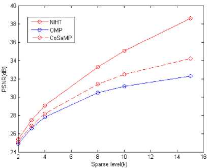
Fig.1. Comparison of the Algorithms at different sparse levels, PSNR vs k

Table I and Table II represents the performance measurements in terms of PSNR and MSE respectively. In both tables, Sparsity level k is varied from 2 to 15 and the corresponding values of PSNR and MSE of the three algorithms i.e., OMP, CoSaMP and NIHT are recorded. As observed, NIHT gives higher PSNR and lower MSE values compared to other algorithms for each sparsity level.

Table III depicts the results of noise performance of these algorithms for different images. Noise analysis is done by the addition of noise of varying variance, σ . The value of σ is varied from 0 to 2, in steps of 0.5. The NIHT algorithm provides better results by delivering higher PSNR among all these algorithms.

Fig.1 represents the graph of comparison for three algorithms at sparsity level k = 2, 4, 8, 10, 15. From this graph, it is observed that the NIHT algorithm provides better results in terms of PSNR compared to other two algorithms. For the lower sparsity levels, PSNR value difference between all three algorithms is less but as sparsity values increases, this gap also increase and makes the NIHT algorithm superior.

Fig. 2 represents the MSE comparison between three discussed algorithms for different sparsity levels. As shown, MSE values are lower for the NIHT algorithm as compare to other two. Hence, the NIHT algorithm provides better reconstruction as compare to other two. Fig. 1 and Fig.2 graphs are plotted based on the results obtained on Boat image and similar graphs can also be obtained for other images.

Fig.3 represents the Noise performance comparison among the three algorithms, i.e., OMP, CoSaMP and NIHT. It is clearly visible that noise performance of the NIHT algorithm is far better than other two, as PSNR approaches to higher values compare to other two methods.

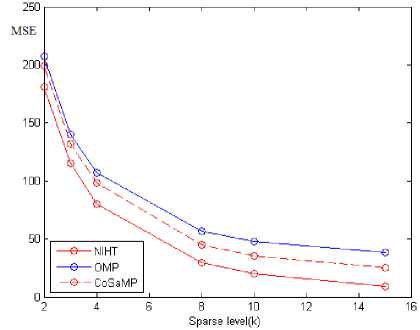
Fig.2. Comparison of the Algorithms at different sparse levels, MSE vs k at noise level σ =0.5

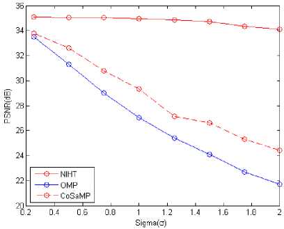
Fig.3. Noise performance of algorithms for various noise levels at k =10

(d)

(e)

(g)

(h)

(i)

(a)

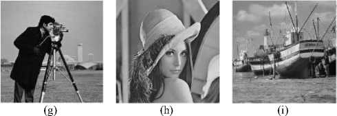
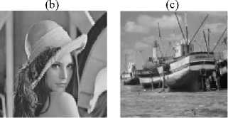
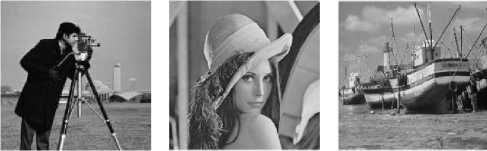
Fig.4. Reconstruction by OMP:(a) Cameraman image (b) Lena image (c) Boat image (d), (e), (f) Reconstructed images for sparsity level, k = 2 (g), (h), (i) Reconstructed images for sparsity level k = 8

(d)

(e)

Fig. 4, Fig. 5 and Fig. 6, shows the reconstruction of images at different sparsity levels for three algorithms. Here, results of cameraman, lena and boat images are shown, though similar results can also be obtained for other natural images. Though algorithms are able to reconstruct images at very low sparsity levels, satisfactory results can be obtained for higher levels. High PSNR values at higher sparsity levels reflects the fact that it has more points to estimate the vectors properly as compared to lower levels. From theses images, it is found the NIHT algorithm provides better subjective results compared to other two methods.

After evaluating algorithms on the basis of pixel difference measurement parameters, they are also evaluated on the basis of Human Visual System (HVS) parameters, i.e. , Structural Similarity Index (SSIM), Universal Image Quality Index (UIQI) and Mean SSIM (MSSIM). Table IV represents the comparison of above mentioned HVS parameters for all three algorithms for cameraman image.

(g)

(h)

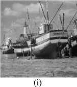
Table IV. Measurements Of Hvs Parameters For Cameraman Image

HVS Parameter	k	OMP	CoSaMP	NIHT
SSIM	2	0.87	0.87	0.88
	4	0.9	0.91	0.93
	8	0.92	0.94	0.96
	10	0.93	0.94	0.96
	15	0.93	0.95	0.98
UIQI	2	0.68	0.68	0.76
	4	0.72	0.73	0.83
	8	0.75	0.77	0.88
	10	0.75	0.78	0.89
	15	0.76	0.8	0.91
MSSIM	2	0.96	0.96	0.97
	4	0.98	0.98	0.99
	8	0.98	0.99	0.99
	10	0.99	0.99	1
	15	0.99	0.99	1

(a)                         (b)                         (c)

As shown in Table IV, the performance of the NIHT algorithm is better among other algorithms, as it offers higher SSIM, UIQI and MSSSIM values.

• V.    Conclusion

In this paper, the concept of Compressed Sensing is reviewed and image reconstruction is carried out using OMP, CoSaMP and NIHT algorithms. Based on the experimental results, it is observed that the NIHT algorithm provides better noise performance compare to

OMP and CoSamp, whereas OMP and CoSaMP are almost equally efficient in the image reconstruction without noise. The NIHT algorithm offers higher values not only for Pixel Difference Measurements, PSNR and MSE but also for Human Visual System (HVS) parameters, SSIM, UIQI and MSSIM.