A speaker recognition system using gaussian mixture model, EM algorithm and K-Means clustering

Published Online November 2018 in MECS DOI: 10.5815/ijmecs.2018.11.03

In our daily life, body language, text language, image language, and speech are the many forms of communication. However, these forms of speech are always regarded as the strongest forms because of their rich dimensional characteristics. The speaker's gender, attitude, mood, health status, and identity also refer to a rich dimension apart from spoken and written language. This information is of the utmost importance to effective communication in today's life.

The development of speech is a study of word signals and methods for developing different speech signals. Voice action can be considered as a particular case of digital signal sort out because the signal is typically digitized and applied to speech signals. The word processing aspects include acquiring, processing, storing, transmitting, and outputting speech signals. The signal input is called speech recognition, the speech is called synthesis. Word signals are mainly divided into three parts:  speech recognition, speech recognition, and speaker recognition [2].

• A.    Human Speech Production System

Human's uses spoken the language to communicate information which is the most natural. The speech signal transports not only what is being said but also realize personal unique attributes of the speaker. Speaker's specific characters are derived from two components, which are the physiological and behavioral attributes of the speaker. Understanding the behavior of speech construction will help to identify more successful techniques to isolate the characteristics of the speakers. The representation of members of human's voice creation. From a physiological perspective, speech is produced by an excitation production process. This process works when human is excited to speak, lungs consume the air in it and transfer that air to the vocal tract. The excitation medium of the improvised and undirected speech related to air current, causes the sound path to resonate, resulting in resonance in its characteristic frequencies (difficult frequencies). The vocal canal begins at the time of vocal folds open and finishes to the tip of lips. The system contains three main features, which are the pharynx, cavities like oral or nasal. The frequency of the formula is determined in the form of the acoustic channel, depends on four organs tongue, lips, jaw, and throat. By this characteristics, we control the voice and produce the speech.

• B.    Speaker Recognition System

Speaker recognition is used for recognizing or identifying from persons individual sound by machine. The system may depend on the text (trained and tested for a particular word or phrase) or independently of the text (without limiting the content). The speaker identification or verification are categorized by depending on final task or decision of machine. Easy-to-access, natural and microphones (inexpensive devices) are used for collecting data is to perform the process of specific applications which are referenced to speaker recognition. The claimed speaker tracking is to locate a given talker's segment in an audio clip or in an automatic teleconference segmenting by potential applications for speaker identification in multi-user systems. In addition, it found it useful in helping the court to discuss and court-applied transcription [7]. In speaker recognition technology, feature extraction is mainly used. Extracting features is a process of holding useful statistics of data from a speech signal while eliminating unwanted signals such as noise. Here, the conversion of the original acoustic wave into a tightly packed representation of the signal feature selection technique. The series of eigenvectors representing a close-packed speech signal is determined by a feature extraction method. The feature vectors extracted from the original signal in the feature extraction module prominence speaker-specific attributes and vanquish statistical redundancy [9]. This system will perform operations in three phases which are a preprocessing phase, the training phase, and decision phase.

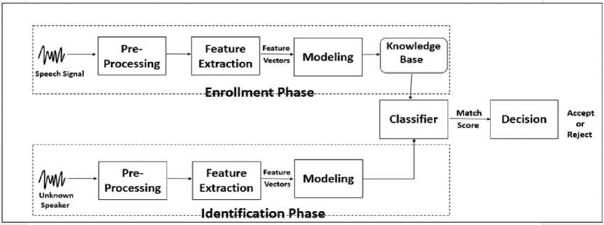
Fig.1. Block-diagram of Speaker Recognition system.

The outputs of the pre-processing phase will be the speech attribute were extracted from the given speech wave. This process is called an extraction feature. These withdraw features will be used for the training phase to train the system. Throughout the decision-making stage, an unknown speech will be compared or tested with the speech given in the system. A particular speaker will be identified by matching the percentage of the speech with the unknown threshold for speech training. If the match rate is greater than the threshold, only the person's ID will be displayed, otherwise the message "Person not available" will be displayed.

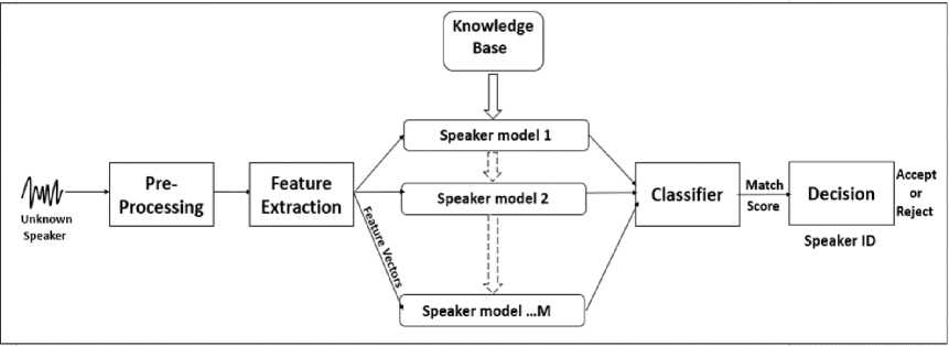
Fig.2. Speaker Identification system.

The checking, verifying and identifying are key applications for identifying speakers. The verification or authentication name is the voice used to verify the certain identity by declared speaker's voice print or vocal tract. On the further work, the task of identifying the speaker is unknown, known as identicalness. In a sense, the speaker validation is a 1: 1 equivalent where the sound of a speaker is equal to one speaker model also called "audio print" or "audio form", while the definition of the speaker is an M: 1 match where Compare the sound against the speaker model M [7].

• II.   R elated W ork

A study of existing theories and practices (literature) in the speech signal processing and machine learning area or domain helps to know about it more deeply. It also helps in the identification of gaps in signal processing for speaker recognition system and in scoping the study by identifying its limitations and assumptions. All this helps to draft the problem statement.

• A. Revathi et al. [17] proposed a text independent and text-dependent speaker recognition using frequentative clustering approach. The clustering model developed on training speech samples for better accuracy by using MF-PLP (mel-frequency linear predictive cepstral) as well as PLP (perceptual linear predictive cepstral). This is system performs for different purposes like speaker identification and continuous speech verification. The model is clustered using a K-means algorithm. They compared the results between MF-PLP and PLP for predefined text and independent text speech.

The authors Tomi Kinnunen and Haizhou Li [1] implemented an independent voice remembrance technology, with an important on text-independent placement. He has done work on speaker recognition actively for nearly ten years. The author provides important aspects of a survey of classical as well as an art in various sate methods. The beginning stages are the basics of independent speaker remembrance, with regard to speaker modeling technique and feature extraction method. The advanced computational ability of the technique to handle durability and cycle variability. The progression of vectors so as to approach super contains a new explosion of feature and reprints the trend of methods. It also provides detail information about current developments and discusses the methodology for assessing speaker recognition systems.

Qing, et al. [2] they introduce a system to ameliorate the successfulness of feature parameters, a weighted feature extraction method. The Ear recollection is a type of biometrics methodology, which is most favored and mostly used. Regulates the average contribution sequence and analyzes each component of the LPCC. Construct on the series, LPCC weighs by every proportion to produce a pressure on feature variables. Matlab implemented the environment of the LPCC properties of the speaker remembrance system which is under. The experimental results of the speaker recognition system show the best presentation than the existing models.

In paper [4], JunzoWatada and Hanayuki proposed an HMM as an emotional classifier to perform the testing process using voice info. Voice signal is a flexible way of communication, also it is useful where each signal has different frequency characteristics and levels. Many problems were faced while determining sounds, such as pitch, speed, and exactness of processing audio features. The experiment was motivated to identify and inspect human speech in a more than one speaker background environment of connecting or accidental conversation. And to analyze and verify human voice research was motivated mind, the environment is a multi-speaker meeting conversation or accidental.

Asma, Mansour, and ZiedLachiri [6] they highlight a systematic view of identifying the amplifiers under several emotional conditions based on the multi-vector support seed machine (SVM) workbook. Strengthening the performance of the process of recognizing the emotional speaker has received increasing attention in recent years. The author compared two methods to extract features, to obtain the best accuracy features are used to present a psychological speech in sequence. They used two methods first method is the MFCC and another method is SDC both are merged with MFCC (SDC-MFCC). This two method were processed by mean and variance attribute. Experiments are performed on the EMOCAP database using two multi-layered SFM approaches one against all (OAA) and one against one (OAO). The outputs obtained shows that SDC-MFCC is superior to ordinary screwdriver performance.

In paper [9], N. Singh, et al. author discussed three main areas of speech technologies which are authentication, surveillance and forensic speaker remembrance. The goal of this research is to introduce the same specific areas where the speech recognition system is used. We also get the information about all application which is related to speech recognition.

The authors S. Paulose and A. Thomas [10] introduces an automated speaker endorsement technique which identifies the person from the feature coefficients included in the speech signal. The proposed system is applicable to several security application. The matching results of this system are based on the techniques used to sort the coefficients from the speech signal, the techniques for model making and the classification technique were used to identify the speaker from training as well as the testing dataset. Gaussian model is used for modeling i-vector features on the basis of short utterance and long utterance. Here the research of identification systems is experimented using two feature extraction techniques spectrum-material features as well as soundsource features. The i-vector method is implemented on two different classifiers and the accuracy results are compared.

• III.    P roposed M odel

The methods and models used in speaker recognition system are discussed below.

• A. Pre-processing Technique

The pre-processing technique contains silence removal, noise removal and pre-emphasis [20].

• 1)    Silence Removal:

Silence removal is used to eliminate the unvoiced and silent portion of the speech signal. For this, the segmentation (framing) is performed on the input voice signal. And each and every segment is compared with a threshold value. After normalization, the silence should be removed for better results by setting the threshold to 1% (0.01). Silencing is performed in the time zone on speech samples, where the amplitudes are thrown out which are below the sample. This process gives speech samples smaller and less duplicate of other samples by improving the performance of recognition [20] [21].

• 2)    Noise Removal:

The aim to use it for eliminating the background noise from the speech signal. We used a band-pass filter to clean the noise from the speech signal. The band-pass filtering set the default range for the signal is [1000 Hz, 2853 Hz] frequency. In this, the signal flows between default frequencies. The below than 1000 Hz and higher than 2853 Hz frequency is trimmed [20].

• 3)    End-pointing:

The end-pointing algorithm is used here, to eliminate the edges, local minima, local maxima and continuous equality points from the sample points of the speech signal. By using this algorithm we reduce more unnecessary points and increases the accuracy [20].

Algorithm: End pointing elimination.

The peculiarity of the statement includes the reduction of the number of resources or weights required for a large number of data descriptions. Most serious problem is the count of features that make a complex data analysis. Examination with a wide number of variables mostly needed large memory and computational power as it can lead to a classification algorithm that is more appropriate for sophisticated and circulating samples for the current sample values. The peculiarity of removing is that the general term of methods for focusing on variables to obtain this problem is still quite accurate.

• 1)    Mel-Frequency Cepstral Coefficients (MFCC):

The activity of sound contains the mel-frequency cepstrum (MFC) assigns the small-range energy spectrum of the voice, related to the sequential cosine conversion of the logarithm capability to the nonlinear frequency scale of the frequency.

Input: S = { S 1 , S 2 , S 3, … Sn } Set of n Speech Samples.

Output: N = { N 1 , N 2 , N 3 ,… Nn } Set of new trimmed n Speech Samples.

• •    Begin

• •    Initialize

o   S_p ← Sample points.

o  Tr ← Threshold value o  Sr ← Silence removed o SE ← Start and End point o  Lmin ← Local minimum o  Lmax ← Local maximum o   Ce ← Continues equality points

• •    Begin

• •    for ( S i in S) do

• ■    while ( S i != null) do

• •    Apply pulse code modulation.

• •    Get S p.

• •    Remove noise from S i.

• •    Eliminate silence from S i.

o Set T r = 0.01

o    if ( S p <  T r ) then

• ■    Eliminate those S p.

o    else

• ■   Get S p.

o   end if loop

• •    Apply end pointing on S p.

o   Find SE, Lmin, Lmax, and Ce and eliminate them.

o    Get S p.

• ■    end while

• ■    for ( N i in N) do

o  Ni = Si end for loop

• •        end for loop

• •        end

• B.    Feature-Extraction Technique

4#—* Speech Signal	Framing	—•	Windowing	.—,	FFT
				Magnitude		Spectrum
MFCC ----	DCT	*—	LOG Energy	*-------	Mel-Seale

Fig.3. Block diagram of Mel-Frequency Cepstral Coefficients (MFCC)

Mel-frequency cepstral coefficients (MFCC), which together form MFC. File filter bank energy DCT is the final step to calculating. The filtered banking energies are quite interconnected with one another, as our filter banks are totally the same. The meaning of the covariance matrices of diagonal values is that the DCT Decor refers to the energies that can be used for model models. MFCC is regularly used as a parameter in sound recollection systems. MFCC is used to recognize spoken word by telephone automatically. MFCCs are also used in music lyrics as classification and measure the audio similarities. The overall operation of MFCC describes as below [7].

• •    Framing: The speech signal is divided into several blocks at the particular duration of 25-30 ms which are frames. The signal is separated into (p) number of samples and frames are segmented by (s), where (s) is less than (s). In 20-30 ms the voice of human is constant, so we make the frame up to 30 ms.

• •    Hamming Windowing: Each and every frame in preprocessing phase is multiplied with the hamming window sequentially to maintain signal continuously. For eliminating the discontinuity the window function is applied. The window is used to make zero at the starting and ending of each frame which reduced the spectral misrepresentation [7].

Y (s) = X (s) * W (s)             (1)

W (s) is the window function.

• •    Fast Fourier Transform: For converting the signals from the time domain to frequency domain, the Fast Fourier Transform is used. By converting into frequency domain we get the magnitude frequency response of each frame. The result we get in a spectrum by applying Fourier transform.

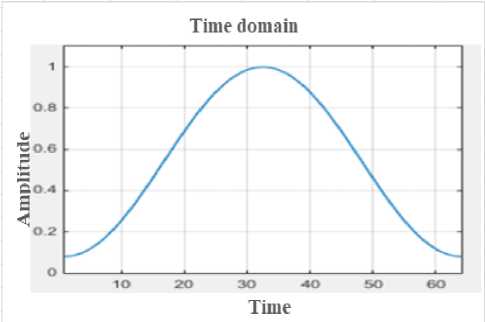
Fig.4. Original Speech signal in the time domain

The Figure 4 is the representation of the original signal graph.

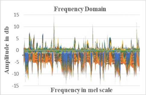
Fig.5. Speech signal in the frequency domain

• •    Filters (Mel-Scale): The filters are used to eliminate unwanted noise or speech. The triangularly shaped filter is mostly used in the preprocessing phase. Fourier transform is used to implement filter bank by transforming window of speech.

• •    Discrete Cosine Transform: This transform technique translates a specific sequence of data points, which is alternate of different frequencies in terms of the sum of the cosine functions. The complexity of DCT is also O(nlogn) [4].

n -1

X = 1V n ∑ x cos( π f ( i + 0.5))/n,       (²)

i =0

Where, f= 0, 1, 2 …, n-1

The Mel-Scale frequency is calculated by multiplying into linear frequency f, which convert linear scale to mel-scale shown in the bellowed equation. [10],

Mel ( f ) = 2595log 10 (1 + ^f )

Thus, the following Figure (Fig.6) represents mel-frequency cepstral coefficient.

MFCC feature vectors

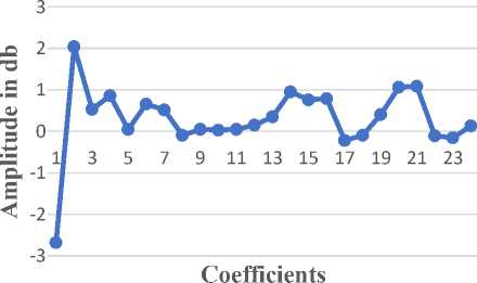
Fig.6. Mel-Scale Cepstral Coefficients

The Figure 6 shows the graph of 24 mel-scale features vectors converted by linear scale frequency. Which are extracted by the Fourier transforming method on raw data. This is 24 features vectors of a single speech signal used for modeling.

• C.    Classification Technique

The classification technique is an important activity in the speaker recognition system. The formulas and description of it are discussed as below.

• 1)    Gaussian mixture model:

The GMM can be seen as an extension of the VectorQuantization model, where groups overlap. That is, the feature vector is not set to the nearest cluster, but has a non-zero probability of the origin of each cluster. GMM is made up of a limited mixture of Gaussian multivariate components. GMM, with k, is specified by its probability density function [1].

This model is a heavy sum of Gaussian distributions capable of determining a random separation of supervision. The equation of likelihood method of a GMM for an examination of x is given as below [10],

M

P(x| λ) = ∑wnpn(x), n=1

The n ^th Gaussian density p ( x ) contains the w as weight [10].

pn(x) =   D/2 11/2.exp{-1(x-µn)∑- (x-µn)}

2πD/2 | ∑n |1/2         2

In the above equation, ∑ _n and µ are the matrices of covariance and the mean vector of the n ^th Gaussian, sequentially.

• a)    Maximum Likelihood Estimation:

MLE’s are the elements of the parameters which increases the probability of the observed items. Parameter estimation for GMM using maximum likelihood, λ denotes an initial model for ML. The mean and variance are estimated from the known data to maximize the likelihood function [15], [19].

Ln { L ( λ | x , x , x ,... x )} = π ⁿ Ln { f ( x | λ )}

It is often more convenient when working with the natural logarithm of the likelihood function. GMM is able to build self-clustering boundaries. The mixture model is a probabilistic data which belong to the distribution of the mixture model. The density function in the distribution of the mixture is a convex combination of other probability distribution functions [19]. Each and every elements component of the mixture is a Gaussian distribution with its own parameters and its corresponding variance variables.

• b)    Expectation Maximization:

This algorithm can be used to estimate the underlying variables, such as those that come from the distribution of the mixture. The EM algorithm is a method to get the maximum probability, evaluates for structure elements when our data is not complete or unexpected. This method is repeated again and again to find the maximum potential task. The algorithm of expectation maximization as below [15],

• •     First, initialize the Я parameters for some

random values.

• •    For each possible value of Z, compute the

probability by given Я.

• •    Then, use calculated Z values only to calculate a better estimate of λ parameters.

• •    Repeat steps 2 and 3 until convergence.

Table 1. Symbols and their description

Symbols	Description
P(P)	For an observation of x the likelihood of GMM model is λ.
µm	Mean vector.
Vm	Covariance matrix.
P m (X)	Gaussian density.
Z	The probability of each possible value.
Ln L ( x )	Natural logarithm of the likelihood function.
P(x)	Mixture components.
W(i)	Weighted coefficients.

The process continues until the algorithm is covered on a constant point by creating a better guess using new values. K-mean algorithm is used for clustering or training the data model.

The Table 1. shows symbols and their description. This table may help to understand the equations easily.

• IV.    E xperimental D etails

The experimentation setup is built on Eclipse IDE using Java programming language, and the training, as well as testing, is performed on 28 speaker’s speech samples of MARF corpus.

• A.    Training and Testing Data

The proposed system performs on 319 training speech samples, and 28 testing speech samples from the MARF dataset [18]. The speech samples are divided into frames into 20 ms durations, by this, we get the constant voice. For smoothing this frames we use Hamming windowing operation. Here, we get 24 feature vectors by applying the MFCC feature extraction technique. And also another property like log-energy and magnitude are extracted. The detail of speech samples and their formats are described below.

• a)    Speech Sample Format [18]:

• •    Audio Format: The wave files are in Pulse Code Modulation audio format (PCM). The speech samples in the dataset contain this audio digital encoding file format which has  (.wav) file

extension format.

• •    Sample Size: The 16-bit audio sample size is used in this system because less bit sample size doesn’t give better results. And more than 16-bit sample size unnecessary increase space.

• •    Sample Rate: The maximum sample rate is set up to 10 kHz. The sampling frequency rate is measured by sample per second in the audio file.

• •    Channels: The 1 (mono) channel refers to the output of sound. The speech signal is arranged in a mono channel format to reduce complications while loading samples process.

• •    Duration: The duration of speech sample is about 8 to 22 seconds.

• b)    Training and Testing graphs:

The following Figures (7 to 10) contains the information about training and testing on MARF dataset. We performed the training and testing process by using two different pre-processing techniques. The first technique is the existing pre-processing technique and second is the elimination of continuous equality points in MFCC. The traditional technique contains silenceremoval, pre-emphasis, and noise removal process.

The traditional technique eliminates silence, noise and boosts the lower range frequency. And in modified technique, it eliminates local edges and continuous equality points. This technique filter-out sample points that are not endpoints. The following Figure 7 and 8 show the resultant feature vectors graph using traditional MFCC technique.

Training Graph j5 5000

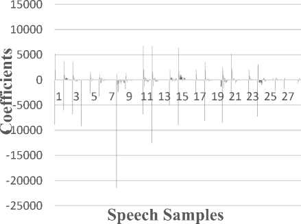
The above Figure 8 shows the testing graph. Here, each speech sample contains 24 different coefficients. The testing graph (Figure 8) represents the extracted resultant coefficients of 28 speech samples before elimination of points, and they are stored in the knowledge base. The coefficients of 28 speech samples before elimination of following Figure 9 and 10 shows the resultant feature vectors graph using the End-Pointing technique.

гм^юсоогм^юсоог^^юсоо t<--5000         HHHHHNMMrsirsm

О

-10000

-15000

-20000

-25000

-30000

-35000

Speech Samples

• ■    C1  ■ C2  ■ C3  ■ C4  ■ C5  ■ C6  ■ C7  ■C8

• ■    C9  ■ C10 ■ C11 ■ C12 ■ C13 ■ C14 ■ C15 ■C16

• ■    C17 ■ C18 ■ C19 ■ C20 ■ C21 ■ C22 ■ C23 ■C24

Training Graph to e 0

oj ^чтшг^.сл’нттг^сл’нттг^сл

-      rsJ’^-lDOO^Hminr^CnrsJ'^-lDOOO

-2000

у-4000

о

U-6000

-8000

-10000

-12000

-14000

-16000

-18000

Fig.7. Training Graph before elimination

The above Figure 7 represents the extracted resultant coefficients of 319 speech samples before elimination of end points and they are stored in the knowledge base. The C1 to C24 are the 24 coefficients shown in different colors. The graph shows the 24 MFCC coefficients for 319 training speech samples.

Testing Graph

■ C1 ■ C2 ■ C3 ■ C4 ■ C5 ■ C6 ■ C7 ■ C8

■ C9   ■ C10 ■ C11 ■ C12 ■ C13 ■ C14 ■ C15 ■ C16

■ C17 ■ C18 ■ C19 ■ C20 ■ C21 ■ C22 ■ C23 ■ C24

Fig.8. Testing Graph before elimination

-20000

Speech Samples

• ■    C1  ■ C2  ■ C3  ■ C4  ■ C5  ■ C6  ■ C7  ■C8

• ■    C9  ■ C10 ■ C11 ■ C12 ■ C13 ■ C14 ■ C15 ■C16

• ■    C17 ■ C18 ■ C19 ■ C20 ■ C21 ■ C22 ■ C23 ■C24

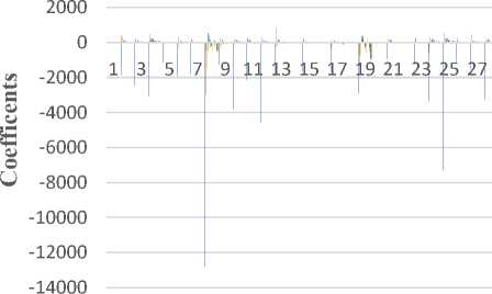
Fig.9. Training Graph after elimination

The above Figure 9 represents the extracted resultant coefficients of 319 speech samples after elimination of end points and they are stored in the knowledge base. The C1 to C24 are the 24 coefficients shown in different colors. The graph shows the 24 MFCC coefficients for 319 training speech samples. As shown in Figure 9 and Figure 10, in the graph of training samples after elimination of end point contains less amplitude of coefficients than Figure 9 By the elimination the computational speed, as well as accuracy, is also increased.

The above Figure 10 shows the training and testing graph. Here, each speech sample contains 24 different coefficients. The testing graph represents the extracted resultant 24 coefficients of 28 speech samples, and they are stored in the knowledge base. As shown in Figure 8 and Figure 10, the graph after elimination gets less number of coefficients with respect to amplitude. And local minima and maxima are also eliminated, by this the computational speed and accuracy is also increased which is shown in the results chart (Table 2).

Testing Graph

Speech Samples

■ C1 ■ C2 ■ C3    C4 ■ C5 ■ C6 ■ C7 ■ C8

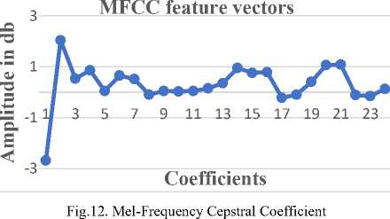
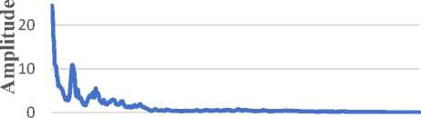
Figure 12 shows the graph representation of the mel-cepstrum coefficients, useful for modeling or training dataset. The 24 MFCC coefficients are extracted from the speech sample.

• ■    C9   ■ C10 ■ C11 ■ C12 ■ C13 ■ C14 ■ C15 ■ C16

• ■    C17 ■ C18 ■ C19 ■ C20 ■ C21 ■ C22 ■ C23 ■ C24

Fig.10. Testing graph after elimination

• B.    Model Training

In this experiment, the GMM and k-mean approach are used. The model training is done by using the K-mean and EM (Expectation Maximization) algorithm on 24 feature vectors for Gaussian selection medium. The endpoint elimination in the pre-processing phase helps to reduce unwanted points and increases computational speed as well as recognition accuracy. On the bases of mean and variance, k-mean and EM algorithms are used for clustering the data. Here, 32 centers are taken to cluster or model the speech samples.

On this coefficients the mean and covariance it calculated by GMM and Minkowski Distance for training or modeling the system. The system is tested on 319 training samples and 28 testing samples of MARF dataset.

The result of end-point elimination technique shows the good recognition accuracy by K-mean and Expectation-Maximization algorithm used in Gaussian modeling. The system is trained on 319 speech samples and tested on 28 speech samples for recognition. The GMM classifier with MFCC feature extraction technique matched 27 speakers out of 28 by eliminating continuous equality points. The system got 96.42% accuracy in the result by the elimination of continuous points. The results of classifiers and their feature extraction technique are shown in the comparison chapter.

• V.    R esults and D iscussion

This system mainly works to extract continuous signal to get MFCC features and trains that by GMM classifier. The FFT is used to convert the time domain signal to the frequency domain. The frame is divided into 30 ms, on that duration we get stationery values.

/N ГМ ГМ Г

Samples

Fig.11. Discrete values of speech

The above Figure 11 shows the graph of discrete value extracted by a continuous speech by using Fast Fourier Transform. Here we get the 512 discrete values for modeling the classifier.

• VI.   C omparison

The comparison between modeling methods and feature extraction techniques in Table 2. as below.

The author S. Paulose et al. [10] introduces the GMM modeling technique with two different features Inner Hair Cell Coefficients (IHC) and MFCC. For this two feature, they got 81% and 96% accuracy respectively. Another form of speaker recognition introduced by H. Veisi et al. [4] by using HMM and MFCC in a multispeakers environment. The Alsulaiman et al. [9] produced a technique that adds new samples without changing sample features. And the MFCC features were extracts and modeled by GMM gives accuracy up to 91.41%. In paper [24] the author introduced modified grouped of VQ for modeling using 16 MFCC feature vectors performs 90% exactly for recognition of speaker. The estimation of EER on both genders is done in the paper [11] by N. Dehak et al. For this results the MFCC and Delta coefficients are merged for Gaussian modeling. The author M. Alsulaiman et al. [14] introduces MDLF (Multi-Directional Local Feature) which works on Arabic language phonemes to find the recognition rate.

Table 2. Comparison Of The Proposed Method With Literature.