A Stochastic Model for Document Processing Systems

Published Online September 2016 in MECS DOI: 10.5815/ijieeb.2016.05.07

With the development of Internet, e-commerce and egovernment, the workflow of complex documents processing in an organization become a problem of great scientific, technical and economic interest. The purpose of this work is to propose a mathematical formalization of the problem and analyze the key performances of systems for which the basic assumptions we make here can be matched.

A great amount of research has been devoted to workflow technologies (see for instance [6], [2], [3], [18], and the many references contained there). This activity has produced numerous tools available in the software industry. However, this work was essentially focused on workflow modeling using Petri nets with constraints. From our knowledge, very few attention has been given to performance measures of modeled systems. These measures become even more important when human beings play a key role in the workflow process. The performance analysis is indeed necessary when the workflow is related to a document processing system in public and private administrations because the system load has a huge impact on the processing speed (see [8], [19]). Indeed in such a system, there might be many actors with enough skills to process a given document. The system should thus be able to choose the right resource by taking in account its load and its processing time. Similarly, when a document is introduced in the system the path it follows should benefit from apriori knowledge about how the system behaved for similar documents. System metrics are thus necessary in order to enhance the decision-making process. Van der Aalst ([3]) suggests the use of stochastic models and especially waiting-lines to carry out this analysis on the tactical level.

This paper shows how stochastic methods can be used to represent a system and forecast its behavior using the analysis of exchanged data flows. It should also be noticed that Petri nets cannot capture all the information related to time. Time is involved locally and globally in a document processing system. The service time at each node will affect the waiting line on the next node. In a few well-documented cases, the performances of networks of queues are well studied. These metrics can thus be used to quantify the quality of a document processing system. The context will be clearly defined in the next section. This will lead to a formal model described in section 3. It has a static component which can be seen as a graph and contains all the information about the transition logic, and a dynamic component which can be seen as a network of queues. Useful measures to assess the system quality are derived from this double representation. Basic and more advanced material about Petri nets can be found in [1], [2], [3], [4], [5] for instance. Networks of queues are treated for instance in [7], [12], [13].

• II.    Definitions and Preliminary Results

• 2.1.    Basic definitions

In this section, we shall first state the basic definitions used in the field of document processing systems. Then the main problem linked to document processing will be stated and pictured using a basic example. Eventually, our basic model enabling the analysis of system’s performances will be described and the problems raised by this model will be underlined. This model has two components: a static graph describing the organizational aspects of the document processing system and a dynamic component based on a Markov chain which describes it’s time evolution.

To better understand the problem posed in this paper and the model we propose, we will first define some concepts used thereafter.

Definition 2.1.1. (Management unit). A management unit is an organized group of people working together for a common goal. This can be collaborative work group, team, service, business, administration, institution, public or private organizations, etc. By the term ‘‘organize’’, we mean the existence of a relationship between the people in the managerial unit (e.g. hierarchy). A managerial unit can be perceived as a living organism interacting with its environment, and in which, internal interactions take place. As part of this study, both internal and external interactions are realized through the documents produced and exchanged. Subsets of managerial units are considered as full managerial units; it is the case for services in a general direction of a public administration.

Definition 2.1.2. (Document). A document is a medium (paper, digital, etc.), carrying information that may be exchanged. This can be a letter, a report, a book, a record, a manuscript, a file, or an aggregate of documents. Documents relevant to our study are those that are exchanged within or with a managerial unit.

Definition 2.1.3. (Processing). To process a document is to use (analyze, read, write, modify, etc.) this document in order to extract information or to produce content that will be included in the document.

Definition 2.1.4. (Processing time. Service time. Waiting time). The processing time (denoted T_P) of a document is the sum of the durations for which the station actually processes the document, called service time (denoted T S ) and the time during which the station waits for the other stations to discuss the document before it is returned, called waiting time (denoted T W ).

Definition 2.1.5. (Station or processing unit). It is in a managerial unit, a person (or expert) equipped with all amenities, capable of processing documents.

Definition 2.1.6 .(Document transmission). This is the process by which a station sends a document to another station, optionally specifying the nature of the treatment to be applied.

Definition 2.1.7. (Document processing graph). A document circulates between stations of a managerial unit for treatment. The complex path that it follows can be modeled by a connected graph. More precisely:

• •    The nodes are the processing stations to which the document is transmitted;

• •    Each oriented edge (x, y) is the link between two stations x and y, with the meaning that the document can be transmitted from x to y.

• 2.2.    Main problem

Definition 2.1.8. (Organigram). This is a graphical representation of the relationship between the various actors in a management unit. It shows, graphically, the organization of the management units; that is to say the way in which its various organs are located relatively to each other. The structure allows especially showing hierarchies between the different members of a managerial unit. Reduced to the problem of document processing, the representation of a chart can be made in the form of a directed graph whose nodes are the processing stations, and each edge (x, y) indicates that the node x can transmit a document to node y. The nodes x and y are so-called neighboring.

Definition 2.1.9. (Document tracking). This is the procedure to monitor a document processing graph.

Document processing plays a central role in the daily managerial units to the extent that it is the main occupation of certain jobs. Their treatment results in a flow of information, whose size is growing, especially with the widespread adoption of digital technologies by managerial units. Supported by computers, this flow escapes human operators who are responsible for monitoring the processing of documents without suitable tools. Analysis and mastering of this flow would lead to better monitoring of documents treatment, in particular with the identification of inertia sites and bottlenecks, but also by the control of system capabilities and predicting of its behavior under certain conditions. However, analysis of these data streams can be performed through the development of a mathematical model to represent and predict its behavior. It is from this model that can be derived measures that may lead to metric system performances. However, such a model does not exist in relation to the state of the art. This is why the present paper attempts to fill this gap by proposing a modeling of the data stream generated by the processing of documents, which can be used to develop applications for smart monitoring of treatment of documents.

To illustrate the problem of multiple interactions and data flows generated by the processing of documents, take as an example, the management of cash withdrawals to fund a bank branch (figure 1 and 2). At a time of day, n clients Cl_i , 1 ≤ i ≤ n , from a bank branch form a queue to enter the body C (case 1). The bank offers k boxes, and the client Cl₁ in the lead goes to the first available cash C_i (case 2). However, for certain amounts, any cashier C’_i must seek the agreement of a manager M , before which other cashiers may already be waiting (case 3). There are a total of m managers in the bank. Each manager M’ i must refer to a Branch-Manager ( BM ) for an agreement to withdraw a certain amount. The manager can find other managers pending before the Branch Manager (case 4).

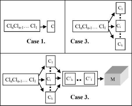
Fig.1. Three document processing workflow examples.

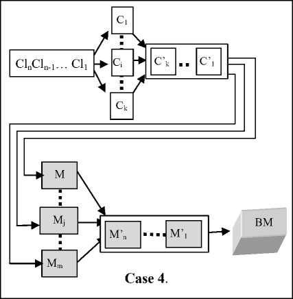
Fig.2. Another document processing workflow example.

This scenario may have loops if we admit that a cashier can become a customer, or a manager can replace a cashier, or if the Branch-Manager replaces a manager. In addition, a cashier can return repeatedly the same document to the Manager in relation to the requirements of various actors or business rules; the same for the manager with his Head of Agency ( i.e. Branch-Manager). This means that the entries in the various queues depend not only on arrival in the system ( e.g. customers) but also on outputs returning the system queues, creating loopeffect. But this loop-effect is systematic in the process of document processing and generates what is considered by users of public services such as delays, with the added bonus of double difficulty to precisely locate the document in its processing graph and estimate the remaining processing time.

Thus in the above scenario, customers will only have the option of undergoing processing time caused by the exchange of information between cashiers, managers and Branch Manager; knowing that there is no tool to control the situation, in particular, to detect blockages and burdens generated by the system. Beyond this anecdotal example, the general problem of document processing, knowing that in practice, in a digital document processing, it is not the agents that move but the documents are transmitted from a processing station to another.

• 2.3.    Modeling requirements

Given the pattern of flows between workstations, the graph is the appropriate mathematical tool for modeling the interactions generated by the exchange of information between document processing stations. Therefore, the subsystem involved in the processing of a document can be modeled by a graph G = ( 5 , E ), where S is a set of vertices (nodes, stations) and E a set of edges (arcs, transitions), that is to say, pairs of oriented vertices ( a , b ) G S 2 , such that can send a document to b for treatment, or b may seek from a necessary information for the processing of the document. This static graph resulting from the organizational structure of the managerial unit is often enriched with additional connections derived from local networks that interconnect the processing stations. Therefore, G represents a system composed of a set of document processing stations (nodes) interconnected by a local network, where each connection represents an arc between two nodes. The link between two nodes reflects the fact that those stations can exchange documents or information required to process documents.

During its processing, the document goes from a node (station) to another, following administrative, technical or business rules modeled by the arc values. Since when a document is sent to another station, this station can be busy or waiting for extra information, one can consider that the document enters a waiting line. Thus, one way to capture this fact is to define a queue W for each station x , which stores the documents it receives until they can be processed. So that when a station x receives a document, it is inserted into its queue W . The station processes a document , which is at the top of the waiting line, the bottom or any other rule stated in the definition of the waiting line. The processing is performed in a random time T ( W , d ) depending on the nature of the document, and the processing unit skill. Information that can be expected from other stations has an impact only on the waiting time. At this level, no assumption is made about the nature of the document processing. After processing, the station sends the document to one or many successor stations according to the graph G = ( S , E ). Among the possibilities, it can either:

• •    close the document,

• •    send back the document to the sender station,

• •    send the document to other  stations for

competence; each transmitted copy will be treated as a full document,

• •    seek information from successors; the waiting time for this information is added to the processing time.

Each document is pinned the total time of processing and waiting it has suffered. Three problems arise when modeling data streams with a static graph. The first is to determine the variables that measure the performance of each treatment plant and the entire system. Among these variables, we have:

• •    A station's load: it is the number of documents being processed or waiting at this station;

• •    The system load: it is the number of documents in the system;

• •    The mean processing time per station, which enables to measure the efficiency of the given station;

• •    The mean total processing time for a document in the system;

• •    The estimated time for a document processing;

• •    The position of a document in the system;

• •    An estimation of the remaining time for a

document processing;

• •    The productivity of a station:  number of

documents treated by time unit;

• •    The speed of a station: mean processing time for a document when all the required information is available;

• •    Station saturation: when the number of waiting

• documents tends to its maximum;

• •    System saturation: when the number of waiting

documents in the system tends to its maximum.

The second problem is that a static graph does not represent the dynamic nature of data streams. For this purpose, queues are required. In addition to the static graph, several dynamic graphs modeling processing steps for a document are required for a full description of the system; which leads us to a multi-graph.

Finally, the entries in each station depend on the output of the stations they are linked to. Since these outputs depend on a random service time, their flow can be modeled by a transition probability between two states of a Markov chain. In this model, each processing unit represents a state of a Markov chain for the document. s etting ( x , x ,..., x ) the sequence of transitions for a document, this amounts to making the assumption that:

P ( X n + 1 = X n   X n = X n ) =

P(Xn+1 = xn+1 I Xn = xn ),(Xn -1 = xn-1),-,( X1 = X1», where X is the stochastic process which represents the sequence of nodes.

• III.    The Formal Mathematical Model

• 3.1.    The general model

• 3.2.    The static model

Static and dynamic description of a document processing system requires the precise mathematical definition of the objects we will handle, mainly graphs and Markov processes. This is also made necessary by the fact that we wish to derive performance metrics.

These will rely on probabilistic calculus under very few regularity assumptions on the model. In the next subsections, we will describe the general model (the big picture) then focus on each component, the static model, and the dynamic model.

The mathematical model described hereafter is meant to capture the systems static and dynamic behaviors including the sequence of possible transitions. Its static component is a graph in which nodes model the states of a Markov-chain and its edges model transition probabilities between states. The static components properties are thus described by the set of states and the transition probability matrix. It should be noticed that these states and probabilities are related to a kind of documents. The system is assumed to handle many kinds of documents.

The dynamic component is a network of queues. A queue is defined for each vertex of the static graph. Its properties are described using Kendall’s notation. The system will thus be formally described by ( S , E , F ) ; where S is the set of processing units, E the set of edges and F the set of waiting-lines (one by a processing unit). In order to make this precise and derive quantitative measures, each component is furthermore described hereafter.

Let G = ( S , E ) be the system graph, where S is a set of nodes and a set of vertices which can be seen as pairs ( a , b ) G S x S . The nodes represent document processing stations, and the vertices, possible transitions between processing stations. The valuation on vertices enables to quantify the cost of a transition from one station to another. This valuation can be a vector. For such a graph, a waiting line W is defined for each node x for which x is a customer. This waiting time represents the time required to process previous tasks when many tasks have to be performed by the station. From the previous definitions, the following relationships can be established for a document d :

T p ( d ) = T w ( d ) + T s ( d ) (1)

Where T , T and T refer respectively to processing, waiting and service times (see def. 2.1.4).

• 3.3.    The dynamic model

The dynamic model enables to track the systems temporal evolution. It states how long a document has been in a waiting line, for how long it has been processed by the station and where it has effectively been sent after processing. The individual trajectory of a document is an outcome among many possible others. Since this trajectory is random, our interest is rather to derive expectation times or probability bounds for these different values. The available information will consist of the probability transition from one state to the other. Denote P(t) the transition probability between station i and station j, at time t . For each document, what is observed is the outcome of a Markov-chain with transition matrix p = (p(t)),  with (i, j) e{1...m}, where m is the number of states.

The systems performances will be determined by the stationary and transient properties of this Markov chain. The time between two transitions is the output of the time spent in the queuing system related to the processing unit. The transition probabilities can be a priori data or estimated from the observations. These transitions probabilities will act in some way as the transition rules defined in Petri nets. The main difference is that after a transition, the model enters a waiting line.

The waiting line is a birth and death process and also has the markovian property. Given assumptions about the service and arrivals discipline, one can derive average performance rates such as the average number of documents in a waiting line. Queue networks are systems in which single queues are connected by a routing network. In this image, servers are represented by circles, queues by a series of rectangles and the routing network by arrows. In the study of queue networks, one typically tries to obtain the equilibrium distribution of the network, although in many applications the study of the transient state is fundamental. Networks of queues are systems in which a number of queues are connected by customer routing. When a customer is serviced at one node it can join another node and queue for service, or leave the network.

For a network of m nodes, the state of the system can be described by an m -dimensional vector ( x , x ,..., x ) where for all i , 1 <  i <  m , X_t represents the number of documents at node i . The first significant results in this area were Jackson networks, for which an efficient product-form stationary distribution exists and the mean value analysis which allows average metrics such as throughput and sojourn times to be computed. If the total number of documents in the network remains constant the network is called a closed network and has also been shown to have a product-form stationary distribution in the Gordon Newell theorem. This result was extended to the BCMP network where a network with very general service time, regimes and customer routing is shown to also exhibit a product-form stationary distribution. The normalizing constant can be calculated with the Buzen’s algorithm.

Networks of queues have also been investigated using Kelly networks where customers of different classes experience different priority levels at different service nodes. Another type of networks is G-networks first proposed by Erol Gelenbe in 1993. These networks, however, do not assume exponential time distributions like the classic Jackson Network. To summarize, formally an entire description of the system will be given by the static and the dynamic models: (S,E,F,P) a network of queues and (S, P) a markov process with states S and transition matrix p = (p(t)), where (i, j) e{1...m}, and P(t) is the probability of a transition from state i to j at time t .

For each waiting line the following measures can be derived from its specifications:

• V 1: Probability of an empty system P ,

• V 2: Waiting probability P ,

• V 3: Mean number of documents in the system,

• V 4: Mean number of documents waiting to be

processed,

• V 5: Mean number of documents in service (in

processing),

• V 6: Mean time in the system,

• V 7: Mean waiting time,

• V 8: Conditions to reach equilibrium (no strangling).

• IV.    System Performances Metrics

• 4.1.    Key performance indicators

A document processing system must match efficiency requirements. Often this is obtained by tuning a few parameters. In order to make such decisions, there should be global metrics sustained by key performance indicators in order to give a snapshot of the system’s performance at any time. Below, we define a few indicators and give example calculations for a dynamic component modeled by MM1 or MMS queues.

Let a system be modeled with a graph G = ( S , E ) , where S is a set of nodes ( i.e. processing stations) and E a set of vertices, i.e. pairs or couples of directed nodes ( x , y ) e S ², such that X can send a document to y for processing, or x can call from y an useful or necessary information for the processing of a document. Many performance measures can thus be defined:

• I1.    The station load I_x ( X ) (with X e S ) is the number of documents in the waiting line of x , including the one being processed:

1 1 ( X ) = W ( X )| +Ф ( X )            (2)

Where W ( x ) is the length of the waiting line, and ф ( x ) equals 1 if X processes a document, and 0, otherwise (if x is idle).

• I2.    The system G load is the number of documents in the waiting lines or being processed; it is equal to the total summation of the stations load:

I 2 ( ^G ) = 2 * , s' 1 ( * )                    ⁽³⁾

• I3.    The mean processing time per station is the average of the processing times by this station over a given time period. It enables to have an idea of the station's efficiency over a given time period. It is obtained by computing for each station or node x a statistic of the processing times which average is given by:

Where N is the number of documents processed by x for the given time period, and T ( d ) is the service time of document d in the station x (refer to def. 2.1.4 for T definition).

• I8.    Station saturation: when the number of waiting documents tends to it is maximum:

MeanPT ( * ) = — 2 N * T_P ( d )         (4)

N

Where N is the number of documents processed by x for the given time period, and T ( d ) is the processing time of document d in the station x (refer to def. 2.1.4 for T definition).

I4. The mean time of document processing for the whole system S (set of nodes) is the average of the processing times for all the stations for the observation period:

MeanPT ( S ) = — 2 7 MeanPT ( * )     ⁽⁵⁾

Where S is the cardinal of S .

I5. The position of a document d in the system is the set of nodes which have d in their waiting lines:

Pos ( d ) = { * , S / d , W ( * ) }        (6)

Where W ( x ) is the waiting line of the station x .

I6. A station's productivity: it's the maximum number of documents processed by time units:

Pr od ( * ) = Ma* ( N )            (7)

Where N is the number of documents processed by x for the given time unit; we assume that all the time units have the same duration.

I7. The speed of a station: it's the mean processing time of a document when all the information is available. It is the average service time of the N documents processed by x for the considered time period:

StationSpeed ( * ) = — 2 N * T ( d ,)        ⁽⁸⁾

I W ( * )| « K ( * )

Where W ( x ) refers to the length of the waiting line of x , and K ( x ) is the waiting line capacity of node x .

• I9.    System saturation: when the number of waiting documents in the system tends to its maximum at each station:

• 4.2.    Performances example for MM1 and MMS queues

V * , S ,( K ( * ) - W ( * )|) <  £      (10)

Where W ( x ) refers to the length of the waiting line of x , K ( x ) is the waiting line capacity of node x and £ is a given bound.

Table 1. System performances.

Designation	MM1 queue	MMS queue
V1. Probability of an empty system	1 - A	(                  ^ P = S -1 Ak_ + A S  1 0    k = 0 k !    S !t   A I             1   S V	-1
V2.      Waiting probability	A	S A w    0 ( S - 1 ) ! ( S - A )
V3. Mean number of documents in the system	A 1 - A	A 71 + — Pw— ) \   S - A)
V4. Mean number of documents waiting to be processed	A 2 1 - A	P A . Pw S - A
V5. Mean number of documents in service	A	A
V6. Mean time in the system	11 ц 1 - A	If -Tw- 1 ц ( S - A J
V7. Mean waiting time	A ц (1 - A )	P w ц .( S - A )
V8. Conditions to reach equilibrium	1 <  1 ц	А <  1 S . ц

Consider a basic example of a network. Let X be the mean arrival rate, — the mean service time and A = — the

v traffic (mean number of arrivals during the mean time). Let S be the number of servers. The performances are summarized Table 1 hereafter:

v service system

• V.    Conclusion

The model that is proposed here is quite general. The basic components of this model are well studied in the literature and key performance indicators are available in numerous cases. The static graph together with the transition matrix can reproduce the behavior of any Petri net. In this extent, this model is more general than the ones used in the literature. On the other hand, the waiting line component is very important in practical applications. In some cases, the waiting time can even become critical. An extension of this work would be to study the model using common examples such as exponential service, FIFO queue and so on, and derive formulas in these specific cases.

A second extension would be to investigate the relationships between the service process and the markovian transition process which chooses the next node. Many different models can be used efficiently. Using this transition matrix as a tuning parameter can give to the entire process more or less random behavior.

Acknowledgment

The authors wish to thank Gabon Government for funding this research activity, and African Institute of Computer Sciences (IAI), National Institute of Post and Information and Communication Technologies (INPTIC), for their support. We also underline how difficult it is to carry such an activity in sub-Sahara African developing countries.