A Study of Time Series Models ARIMA and ETS

Published Online April 2017 in MECS DOI: 10.5815/ijmecs.2017.04.07

Weather Prediction System is having most complex Systems Equation that can only solve by Computer. Weather Forecasting is an inspiration about future weather. There are various techniques concern with weather forecasting from comparatively easy observation of the sky to extremely advance computerized mathematical Models [6].

A.Objective

The main goal of the study is to research a technique that improves the forecasting estimate of various parameters. We would like to match the forecasting of automatic forecasting methods in predicting the weather parameters such as Rainfall, Relative Humidity, Air pressure and Wind Speed etc. However predicting the weather considers many forms, which mainly depend upon the required applications. The forecasting challenge of weather is equal to very first major difficulty depend on non-linear equations which leads to numerical means and mathematical physics. However meteoric knowledge is tentative (unsure) in nature where knowledge on weather is mostly outlined.

Weather knowledge has the noises and outliers this is why analyzed may not be correct. Noises are the random error therefore we need prepossessing of a Weather knowledge to improve the standard of knowledge for precise weather prediction, or to improve the value of exact data for weather estimation. This paper gives an idea to compare the two automatic forecasting methods ETS (Exponential Smoothing) and ARIMA (Autoregressive Integrate Moving Average) using the data of various weather parameters such as Rainfall, Relative Humidity, Air Temperature , Pressure , Wind speed etc. For convenience the paper provided with some basic definition and background that designates the strategies followed by the analysis of weather data by estimation and verification of varies forecasting methods. The accuracy of various strategies is compared by MAE (Moving Absolute Error), MASE (Moving Absolute Scaled Error), MAPE (Moving Absolute Percentage Error) and RMSE (Root Mean Square Error). We also include the criteria AIC (Akaike’s Information Criteria) and BIC (Bayesian Information Criteria).The methods which gives the best forecast will use for comparison and prediction. As of India Meteorological Department information can even be composed that is over all India climate stations head place of work. In information set we are having the parameters that are: Air Temperature, Rainfall, Relative Humidity and Wind Speed among which we consider one. In this paper ARIMA (Autoregressive Integrated Moving Average) and ETS

(Exponential Smoothing) is use for analysis and predicting weather information that are mentioned above. A Comparative study brings between the ETS and ARIMA Model through SSE, MAE, RMSE, MASE and MAPE also include the criteria AIC and BIC result from the given parameters. Automatic forecasting by ARIMA and ETS is performed by using the forecast, time Date, ggplot2, and Zoo packages in R for Time Series analysis, and also various attributes are predicted by considering Correlations. Efforts are being intense to use statistic Autoregressive Moving Average (ARMA) model to forecast or to predict hydrological information. The ARMA Model is use even as a result of its theoretical base in hydrological Studies.

B.Outline

The paper is organized as follows. Section II gives you study on topic as Literature review on related work. Section III presents some theory and concepts of time series ARIMA modeling and forecasting, used to analyses the algorithm on which our future implementation will based on. Section IV gives some overview about Time Series Concept. Section V provides the detailed analysis of ETS Model and the comparison of proposed models. Section VI gives some suggestions for further research and areas of interests.

• II.    Related Works

• A.    Defination

Around the world weather predicting is one of the most challenging difficulties, due to its practical value in popular scope for scientific study and meteorology. The different methodologies i.e., Statistical Decomposition Models, Exponential Smoothing Model (ETS) and Autoregressive Integrated Moving Average (ARIMA) Model variable Time series and following informative variables etc., is used for forecasting purposes. Several Trainings have taken place among the analysis of pattern and circulation in various parameters in different regions of the World. Regression Analysis could be applied for statistical technique and it should be widely used in several sciences and many other relevant Areas.

• B.    Background

  Agrawal et al. (1980) explained the phenomena for time series regression models for forecasting the yield of rice in Raipur district on weekly data using weather parameters [1].Box and Jenkins (1994), in early 1970's, pioneered in developing methodologies for statistic representing within the univariate case often referred to as Univariate Box-Jenkins (UBJ) ARIMA modeling in this approach of the author [2]. Akaike, H. (1976) an information criterion (AIC) which is used as a parameter estimation to check the performance of Model which gives history for the development of statistical theory testing in time series analysis was studied concisely and it was pointed out that the theory testing procedure is not

  effectively defined as the technique for statistical model identification. The most likelihood estimation process was reviewed and a new estimate least information theoretical criterion (AIC) estimate was introduced [4]. Hyndman, R.J.,& Kandahar, Y(2007). Automatic time series for forecasting: the forecast package for R .Monash University, Department of Econometrics and Business Statistics [5]. Weather forecasts provide critical information about future weather. There are various techniques involved in weather forecasting, from relatively simple observation of the sky to highly complex computerized scientific models (M. Tektas, 2010) [6].An Integrated Approach for Weather Forecasting based on Data Mining and Forecasting Analysis by G.Vamsi Krishna where in this paper the weather data was considered with attributes, such as wind pressure, humidity, Temperature, Forecast and Type, of Visakhapatnam city for a period of 97days. The forecasting experiment was carried out for test, the weather condition for the following 15 days by enabling the ARIMA model to predict the forecasts [7]. An Introductory Study on Time Series Modeling and Forecasting by Ratnadip Adhikari and R. K. Agrawal has given an idea about Time series forecasting as a fast growing area of research which provides many scope for predicting future works. One of them is the Combining Approach, i.e. to combine a number of approaches to improve forecast accuracy. Combining with other analysis in time series prediction, we have thought to estimate an efficient combining model, in future with the aim of further studies in time series modeling and forecasting [8].Prediction Of Rainfall Using Data Minning Technique Over by Pinky Saikia Dutta which describe the model by considering temperature, wind speed, Mean sea level as Predictors. They found 63% accuracy in variation of rainfall for our proposed model. The model can forecast monthly rainfall. Some predictor like wind direction is not included due to constraints on data collection which could give more accurate result. The work can be extended for multiple stations in future. The resulted rainfall amounts was intended to help farmers in making decision about their crop[9].Mahmudur Rahman, A.H.M. Saiful Islam , Sahah Yaser Maqnoon Nadvi , Rashedur M Rahman (2013) consider Arima and Anfis Model and explained how ARIMA Model can more efficiently capture the dynamic behavior of the weather property say, Minimum Temperature , Maximum Temperature, Humidity and Air pressure which must be compared by different performance metrics, such as, with Root Mean Square Error (RMSE), R-Square Error and The Sum of the Square Error(SSE) and author can prove that ARIMA would give the more efficient result than other modeling techniques like ANFIS[10]. Prediction of rainfall using an autoregressive integrated moving average model: Case of Kinshasa city (Democratic Republic of the Congo), from the period of 1970 to 2009 by Dedetemo Kimilita Patrick1, Phuku Phuati Edmond2, Tshitenge Mbwebwe Jean-Marie2, Efoto Eale Louis2, Koto-te-Nyiwa Ngbolua3, There aim is to present study of the test a

model of simulation on the monthly series of precipitations data from the Binza meteorological station of Kinshasa/Democratic Republic of the Congo. After their stationnarization of the Time series, we applied an Auto-Regressive Integrated Moving Average (ARIMA) model into the starting series. There model also makes it possible to predict implication of rainfall on the lifestyle of the Kinshasa inhabitants [11].

• III.    Auto Regressive Integrated Moving Average

  ARIMA Stand for Auto Regressive Integrated Moving Average. ARIMA model was popularized by Box and Jenkins (1976).It is combination of three statistical models. It uses Autoregressive, Integrated and Moving Average (ARIMA) model for statistical information. The ARIMA Model analyze and Forecasts uniformly spaced univariate statistic information, transmission of function data, and intercession information that is done by using Auto Regressive Integrated Moving Average (ARIMA) and Auto Regressive Moving Average (ARMA).An ARIMA Model forecasts a value in a response of time series which is linear combination of its own related past values, past Errors and current past values of alternative Time Series. ARIMA Model aims to explain the Auto Correlation within the information and may applied to stationary and non-stationary statistic. The Model written as ARIMA (p, d, q) where p, d, q≥1.An ARIMA Model corresponds to ARMA after finitely many times differences the data .The elements p and q are the order for Auto Regressive and Moving average Components, because the degree of differencing is written as d. Differencing is usually accustomed eliminated the Trend which may Linear and Exponential in a Time Series.

The differencing order d relates that how many times the method yt must be differenced to become stationary. The prediction method was applied by summing last period’s value with some constant, this indirectly help to estimate the prediction changes on a mean at specific interval of time. Various Transformation Techniques may be used for variance stabilization, e.g.., Box-cox

Transformation, Log Transformations. We can also make use of Auto Correlation Function (ACF) to visualize if the statistic is stationary or not. Auto Regressive indicated the Regression of a variable itself. In ARE Models the forecasting variables is a linear combination of its own earlier observations.

An AR (p) Model is often delineated as:

Y = с + ( 1 Y 1 + p ₂ Y ₂ ... + p _p Y _p + Z_t,       (1)

Where Zt ~ (0, 2), c associate unknown constant term, and ^ ,i=1,...,p, are the parameters of the AR Model .A MA (q) Model is often described as:

Y _t = c+Z _t + 9 ₁ Z _t_₁ + - + 9 _q Z _t__q,      (2)

• A.    Estimation and Order Selection

The ACF and PACF can use for the selection of p, d; q. Auto Correlation is linear dependence of variable with itself at two points in time. For stationary processes, we can define auto correlation between any two observations which can depend on the Time Lag h between them.

The Autocorrelation for lag h is given by:

P k = Corr(y t y t-h ) = ^           (3)

From this equation we define as a (0) is a lag 0 covariance i.e., the unconditional variance of the process. Confounding can defined as the distortion in the estimated measure of association where two variables can result from a mutual linear dependence on other variables. Partial Autocorrelation between     and        after removing any Linear dependence [i7].The par-й lag h autocorrelation is denoted as ϕh,h. The plots of sample ACF and PACF are helpful diagnostic when

Table I. Plots Of ACF and PACF For ARMA Models

MA(q) AR(q) ARMA(p, q) ACF Tail off Cut off, q lag Tail off PACF Cut off, p lag Tail off Tail off selecting the order of an ARIMA Model specifically when data must originated by an ARMA (p,0) model or from an ARMA(0,q) model. This shows that how we can find the model by defining the criteria about plots.

• B.    Auto Correlation and Partial Correlation Models

If the ACF and PACF having the positive (large) values that decreased much slowly with time, this means that d is larger than 0, i.e., it should be done by differencing. We use many other ways to define unit tests to see d. Variety of unit root Tests to see where differencing was needed e.g.., increased dickey- fuller (ADF) and kwiat kowski-phillips-schmidt-shin(KPSS). Here, we are using auto.arima function in R which automatically selects the ARIMA Model. This function uses the KPSS test with the null hypothesis to measures that if the data is stationary. The small p-values than 0.5 recommended the differencing was required. After defining the order we have to determine the parameters of ARIMA, i.e..,c,1,

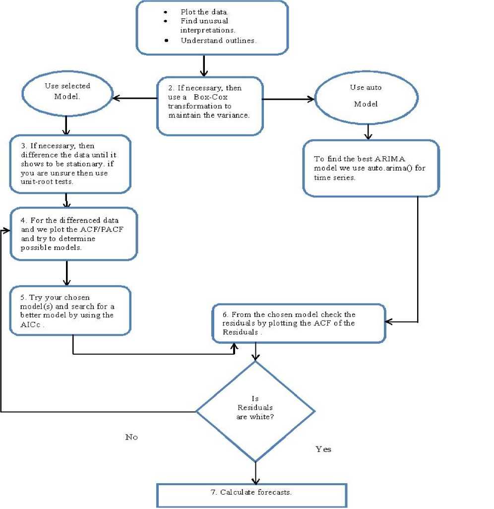
Fig.1. A Flow Chart of ARIMA Model

Where m=p+q+K+1 is the number of parameters in the model and L is the likelihood function. The best model is one with lowest AIC value. BIC (Bayesian Information Criteria) has mathematical formula. It should penalize complexity more than AIC does:

BIC = AI C + log(T) (p + q + P - 1), (4)

Hence final decision about the orders p and q that is probability based on maximum likelihood estimation. It is important to analyze residuals of chosen model for white noise. An approach will be made through minimization of the corrected Akaike’s Information Criteria (AICc).

This can be done by looking at residuals of ACF and formally using it with the value hypothesis that residuals are white noise or not correlated.

• IV.    Time Series

The statistical analysis may be a methodology for constructing effective models by using the values of the parameters which are placed at fixed intervals. The main aim of time series modeling is to thoroughly read about the past observations of a Time Series and then collect them carefully to develop a suitable model which describes the essential structure of the series. One such methodology that deals with time based information is named as statistic modeling or Time series modeling because the name suggested it involves performing on time based information to drive insights to create up-to-date higher cognitive process. Forecasting and Time Series Models are classified into two groups, Univariate Model and multivariate based. A statistic model generally meant to be effected by four main elements, which can be separated from the discovered information. These elements are: Trend, Cyclical, seasonal and irregular elements.

The Statistical Method were practically used because it was multipurpose in various application with the given deployment time. Forecasting is an approach of knowing what may occur to a system in the upcoming time periods. Weather is defined as a time series based data-severe, continuous, dynamic approach [18].

• V.    Exponential Smoothing

  Exponential Smoothing invented by Robert G. Brown’s work as an OR it is analyst for the US Navy (Gass and Harris, 2000). During the Early 1950s, Brown prolonged simple Exponential Smoothing to discrete data and the method should develop for trend and seasonality. Time Series (Brown, 1963), developed the general exponential smoothing methodology. When Time Series forecasted with Exponential Smoothing (ETS) Method, the first order auto-correlation was founded by Taylor in the residuals. Each Exponential Smoothing (ETS) method is equivalently related to one or more stochastic models. It also follows the property of Robustness and treated as a model of judgmental Extrapolation. The idea behind the exponential Soothing is that the forecasts by this approach are the weighted average of past observations and the weight decays exponentially with time i.e.., current observations have larger weights as compare to the earlier ones. Thus produces somehow smart forecasts as compared to the average methods.

We use the simplest exponential smoothing which use to forecast the Time Series with no Trends and Seasonal patterns.

L1/„ = (1 + -

^-(( P p - ^p p-i )^ „+p ^-

^(p 1 - ^p 2 )^ „-1----

Ф р ^ П-р ⁺ @ 1^Z „ ⁺ ’”

⁺ @ q^Z„+1-q ,

Where a, 0< a <1, is the smoothing parameter. We must compare out-of–samples RMSE for the comparison.

• A.    ETS (A, N, N)

Observation Equation defined as:

et = yt- 9t/t-1,

State Equation defined as:

It = It -1 + aZt,(7)

6t = Vt — It — 1 + aZt,

• • Error from single source “because some error process, et”.

For estimating the parameter for minimizing SSE, is to use the strategy of most likelihood estimate beneath the idea that Time Series is Gaussian. The innovation State Space has likelihood function which was computed and maximum likelihood estimate is obtained.

The ETS obtained within the forecast package in R is employ to pick the acceptable model automatically on the premise maximum likelihood method and to seek out the forecast for several steps ahead as needed. Information criteria AIC, AICc, BIC used for choosing the simplest ETS Model among 30 given state space model. In ETS, the default is AICc. The model that minimizes the standard is chosen as acceptable for the information criteria.

AIC (Alkies’ Information Criteria) is:

AIC =-2(L) + 2k,(9)

AICc (Alkies’ Information Criteria Corrected) is:

AICc = AIC + 2(k + 1)(k + 2)n-k,(10)

AICc = AIC + 2(k + 1)(k + 2)n-k,(11)

BIC (Bayesian Information Criteria):

BIC = BIC = AIC + [ln(n) - 2],(12)

MASE (Mean Absolute Scaled Error<1) defined as:

МА5Е=^=1Ы,(13)

MAPE (Mean Absolute Percentage Error) defined as:

MAPE=1Z„=1|ptl,(14)

Where p _t = 100 e_t/y_t .

• B.    Automatic Forecasting Algorithm

  Forecasting Technique is applied to perform forecasting by making the use of ETS function which can

  
  

make use of R. To get a widely and robust applicable to ETS Model for automatic Forecasting are followed:

• 1.    For Every Series, apply all ways that are acceptable, optimizing (both Smoothing Parameter and therefore the initial state variable) of the model in every case.

• 2.    According to AICc value select the best Model.

• 3.    After Selecting the Model with optimized parameter produce the point forecast.

• 4.    To obtain the prediction intervals for the most effective model, analytic results advised by Hyndan [4] and finding α/2 and α/2-1 percentiles of the simulated information at every prediction Horizon.

• VI.    Conclusions

In this paper we have presented a study of the use of Weather Forecasting Techniques with Time Series data. This is very useful since it brings better understanding of the field of Research Analysis and it is present as a vital role during the paper. We focus on performances of ETS Model and ARIMA Model during prediction of different weather parameters such as Rainfall, Air Temperature, Relative Humidity, Gust etc. The Study of forecasting Models which we consider in our paper is ETS Model and ARIMA Model which use for long-range of Meteorological parameters which forecasts could recognize over geographic region and will illustrate a good performance and reasonable prediction accuracy. We have given a Study for Comparing the ETS (Exponential Smoothing) Model and ARIMA (Autoregressive Integrated Moving Average) Model with estimation of MAE (Moving Absolute Error), MASE (Moving Absolute Scaled Error), MAPE (Moving Absolute Percentage Error) and RMSE (Root Mean Square Error). We also included the criteria AIC (Akaike’s Information Criteria) and BIC (Bayesian Information Criteria) values to check which model deploys a best result for Weather parameters.

Acknowledgement