A Study on Discrete Model of Three Species Syn-Eco-System with Limited Resources — (One Period Equilibrium States)

Published Online November 2014 in MECS DOI: 10.5815/ijmecs.2014.11.05

Ecology, a branch evolutionary biology, deals with living species that coexist in a physical environment sustain themselves on common resources. It is a common observations that the species of same nature can not flourish is isolation without any interaction with species of different kinds. Syn-ecology is an ecosystem comprising of two or more distinct species. Species interact with each other in one way or other. The Ecological interactions can be broadly classified as Ammensalism, Competition, Commensalism, Neutralism, Mutualism, Predation Parasitism and so on. Lotka[1] and Volterra [2] pioneered theoretical ecology significantly and opened new eras in the field of life and biological sciences.

Mathematical Modeling is a vital role in providing insight in to the mutual relationships (positive, negative) between the interacting species. The general concepts of modeling have been discussed by several authors, viz., [3-6]. Srinivas[7] studied competitive ecosystem of two species and three species with limited and unlimited resources. Later, Laxminarayan et al [8] studied preypredator ecological models with partial cover for the prey and alternate food for the predator. Stability analysis of competitive species was carried out by [9-10], while Reddy [11] investigated mutualism between two species.

Acharyulu et al [12-13] derived some productive results on various mathematical models of ecological Ammensalism with multifarious resources in the manifold directions. Further Kumar [14] studied some mathematical models of ecological commensalism. The present author Prasad et al [15-22] investigated on the stability of a three and four species syn-ecosystems. Recently, Din et al [23] discussed the basic concepts on stability analysis of discrete ecological models and Kiran et al [24] worked on discrete model of three species ecosystem by considering interactions like prey-predator and commensalism.

The present investigation is a discrete model of three species (S 1 , S 2 , S 3 ) syn-eco system with limited resources. The system comprises of a commensal (S₁), two hosts S₂ and S₃. Further S₂ is a commensal of S₃, S₃ is a host of both S₁ and S₂. Commensalism is a symbiotic interaction between two populations where one population (S₁) gets benefit from (S 2 ) while the other (S 2 ) is neither harmed nor benefited due to the interaction with (S 1 ). The benefited species (S 1 ) is called the commensal and the other, the helping one (S 2 ) is called the host species. A common example is an animal using a tree for shelter-tree (host) does not get any benefit from the animal (commensal).

• II.    Basic Equations Of The Model

The model equations for the three species syn-eco-system is given by the following system of first order non-linear difference equations employing the following notation.

• A.    Notation Adopted

N_i(t)  : The population strength of S_i at time t , i = 1, 2, 3

t      : Time instant ai      : Natural growth rate of Si, i = 1, 2, 3

a ii       : Self inhibition coefficient of S i , i = 1, 2, 3

a 12, a 13 : Interaction coefficients of S 1 due to S 2 and S 1 due to S 3

a23    : Interaction coefficient of S2 due to S3

Further the variables N 1 , N 2 , N 3 are non-negative and the model parameters a₁, a₂, a₃, a₁₁, a₁₂, a₁₃, a₂₂, a₂₃, a₃₃are assumed to be non-negative constants.

• B.    Basic equations

Consider the growth of the species during the time interval (t, t + 1)

• •    Equation for the first species (N):

N ( t + 1) = N ( t ) + aN , ( t ) - a N 2 ( t ) + a₁₂N ( t ) N ₂ ( t ) + a₁₃N , ( t ) N ( t )

• •    Equation for the second species (N 2 ):

N ( t + 1) = N ₂ ( t ) + a₂N ₂ ( t ) - a₂₂N ₂² ( t ) + a₂₃N ₂ ( t ) N ₃ ( t )

• •    Equation for the third species (N 3 ):

N ₃ ( t + 1) = N ₃ ( t ) + a₃N ₃ ( t ) - a₃₃N 2 ( t )         (3)

• •    Species-growth equations in the discrete form:

Consider the nonlinear autonomous system of discrete equations

N ( t + 1) = a N ( t ) - a_nN 2 ( t ) + a₂N ( t ) N ₂ ( t ) + a₁₃N ( t ) N ₃ ( t )

N ₂ ( t + 1) = a N ( t ) - a₂₂N ₂² ( t ) + a₂₃N ₂ ( t ) N ₃ ( t )     (5)

N ( t + 1) = a N ( t ) - a₃₃N ₃² ( t )           (6)

where a i = a i + 1, i = 1, 2, 3

• III.    Equilibrium States

For a continuous model the equilibrium states are defined by dNi = o, i = 1,2,3, the equilibrium states for a dt discrete model are defined in terms of the period of no growth. i.e, N (t + r) = N (t), r = 1,2,3,........., where r is the period of the equilibrium state.

Kapur J.N, Mathematical Modeling through Discrete Mathematics-Fascinating World of Mathematical Sciences, 1989, Volume-II, pp.71-80, Mathematical Science Trust Society, New Delhi.

• • One period equilibrium states (Stage-I)

N ( t + 1) = N i ( t ), i = 1,2,3

The system under investigation has fourteen equilibrium states given by

• (i)    Fully washed out state

E : N = 0, N₂ = 0, N = 0

• (ii)    States in which only one of the tree species is survives while the other two are not

• -      -      - a - 1

E ₂ : N = 0, N₂ = 0, N₃ =----- , when a >  1

a 33

• -       -    a, - 1  -

• E3 : N = 0, N2 =-----, N3 = 0, when a2 > 1

• -    a -1  -      -

• E4 : N =-----, N2 = 0, N3 = 0, when a > 1

a 11

• (iii) States in which only two of the tree species are survives while the other one is not

E ₅ : N = 0, N₂

when a >  1 and a >  1

E ₆ : N = 0, N₂ = a.

a - 1

aa

- a - 1

,N3 = — a33

when a = 1 and a >  1

E7: N1 = — a11

, n 2 = 0, n 3

a - 1

a ₃₃

when a >  1 and a >  1

E 8 ^{: N} 1 = ^a 13

a - 1

V ^a 11 a 33 7

, N 2 = 0, N 3

a - 1

a 33

when a = 1 and a >  1

E9: N1 = — a11

, N ₂

a - 1

, N3

a 22

when a >  1 and a >  1

1 a, -1 ।

E _w: N 1 = a 12 I        I , N ₂ =   --- , N 3 = 0

V a11 a22 7

when a = 1 and a >  1

(One Period Equilibrium States)

(iv) The co-existent states (or) normal steady states

E 11 : N 1

N ( t ) = N ( t + 1) = N ( t + 2) =..................= 0

N ( t ) = N ( t +1) = N ( t + 2) =..................= 0

^a 11

,

N 2

( « 2

—

I a — 1

' 23 I к a33 A

, N 3

a — i

,

a ₃₃

when a , a and a >  1

N (t) = N (t +1) = N (t + 2) =..................=  --- a33

i.e, N ( _{t + r} ) = 0, N ( _{t + r} ) = ^a 3 ^{— 1} where r is an integer and i a 33

= 1, 2

Hence, E 2 is stable.

E ₁₂ : N ₁

^a 11

/      x      I a — 1

(«2 — 1) + a23 I ------- к a 33

I a — 1

+ a13I ------- к a 33

C. Stability of E 3

,

N 2

a ₂₂

( « 2

when a = i and a , a >  i

E13 : N1 = — a11

a — i

к

a ₃₃

, N 3 A

a — i

a ₃₃

N ( t ) = N ( t + 1) = N ( t + 2) =..................= 0

a^ — 1

N ( t ) = N ( t + 1) = N ( t + 2) =..................= -2---

N ( t ) = N ( t + 1) = N ( t + 2) =..................= 0

( a — 1 ) + а^гз

r a3

— i )

+ a_A

N^ = a

a — i

к a 22 a 33 у

( Al a — 1

i.e, N (t + r) = 0, N (t + r) = ——1 where r is an integer and i = 1, 3

Hence, E 3 is stable.

к a 22 a 33 у

, N 3

a — i

a 33

when a = i and a , a >  i

E 14 • N 1

^a 11

I a—1 a12a23 I к a22a33

^N 2 = a 23

a — 1

к a 22 a 33 у

when a , a = 1 and a >  1

к a ₃₃

,

A

D. Stability of E4

N (t) = N (t +1) = N (t + 2) =..................= -J— a11

N ( t ) = N ( t + 1) = N ( t + 2) =..................= 0

N ( t ) = N ( t + 1) = N ( t + 2) =..................= 0

I a — 1

13 I к a 33

a — 1

, N 3 = — a ₃₃

IV. Stability Analysis

A. Stability of E_x ( 0,0,0 )

N (t) = N (t +1) = N (t + 2) =..................=

N (t) = N (t +1) = N (t + 2) ==

N (t) = N (t +1) = N (t + 2) =..................=

i.e, N ( t + r ) = 0, where r is an integer and i = 1, 2, 3

Hence, E_x ( 0,0,0 ) is stable.

B. Stability of E 2

i.e, N ( t + r ) = ^ 1-1, N ( t + r ) = 0 where r is an integer ^a 11

and i = 2, 3

Hence, E 4 is stable.

E. Stability of E5

N ( t ) = N ( t + 1) = N ( t + 2) =..................= 0

N ( t ) = N ( t + 1) = N ( t + 2) =..................

a ₂₂

( « 2

^{— 1 ) +} a 23

a — 1

N ( t ) = N ( t +1) = N ( t + 2) =

i.e, N ( t + r ) = 0, N ( t + r ) =---

^{( a} 2

a — 1

N (t + r) =-----, where r is an integer a33

Hence, E 5 is stable.

F. Stability of E 6

N ( t ) = N ( t + 1) = N ( t + 2) =..................= 0

N ₂ ( t ) = N ₂ ( t + 1) = N ₂ ( t + 2) =

N ₃ ( t ) = N ( t + 1) = N ₃ ( t + 2) =

I a — 1 I

= ^a 23 I           I

V a22 a33 У a3 — 1

, x 1 / i.e, N (t + r) =--- (a — 1)

¹            an _' 1 ^z

^{+ a} 12

' 2     1

a 22

,

a 33

a

N ( t + r ) =   ²

—

I a i.e, N (t + r) = 0, N2 (t + r) = a231 —

—

a 22 a 33

1 |

I ,

a ₂₂

Hence, E₉ is stable.

-, N ₃ ( t + r ) = 0, where r is an integer

a N ( t + r ) = —

—

a 33

Hence, E ₆ is stable.

, where r is an integer

J. Stability of E10

N ( t ) = n ( t + 1) = n ( t + 2) =

a

— 1

G. Stability of E7

N ( t ) = N ( t + 1) = N ( t + 2) =

= ^a 12 I -------- V ^a 11 ^a 22 У

_ ^a2 ^{— 1}

N ( t ) = n ( t + 1) = n ( t + 2) =

= — ( a , ^— 1 ) ^a 11

I a — 1

^{+ a} 13 | --------

V ^a 33

N ( t ) = N ( t + 1) = N ( t + 2) =

a 22

= 0

I a — 1 I             a — 1

i.e, N ( t + r ) = a ₁₂ | ------- I , N ₂ ( t + r ) =------ ,

N ( t ) = N ( t + 1) = N ( t + 2) =

= 0

N ( t ) = N ( t + 1) = N ( t + 2) =

a — 1

V ^a11^a 22 У

N ₃ ( t + r ) = 0, where r is an integer Hence, E 10 is stable.

a 33

i.e, N ( t + r ) = — ( a — 1 )

¹            a_u      ¹

^{+ a} 13

a

N₂ ( t + r ) = 0, N ₃ ( t + r ) = —

a 33

Hence, E 7 is stable.

H. Stability of E8

t₃ — 1

^a 33   У_

,

K. Stability of E 11

N ( t ) = n ( t + 1) = n ( t + 2) =

, where r is an integer

a ₁₁

a ₁₂

a ₂₂

( a

'23 I      3

V ^a 33

I '

^! 13 I ^a

N ₂ ( t ) = N ₂ ( t + 1) = N ( t + 2) =

N ( t ) = n ( t + 1) = n ( t + 2) =

= a 13

n₂ ( t ) = n₂ ( t + 1) = n₂ ( t + 2) =

a — 1

V ^a 11 ^a 33 У

= 0

= — ^(a 2

^a 22

—

1 ) + a 2 ₃

N ( t ) = N ₃ ( t + 1) = N ₃ ( t + 2) =

a — 1

a ₃₃

i.e, N ( t + r ) = a₁₃

a

N₃ ( t + r ) = —

—

a — 1

, N ₂( t + r ) = 0,

N ( t ) = N ₃ ( t + 1) = N ₃ ( t + 2) =

i.e, N ( t + r ) = — < ^a 11

( « 1 ^— 1 )

I a ^{+ a} 131 —

a ₁₂

a 22

— 1

a 33

a ₃₃ Hence, E 8 is stable.

V ^a 11 ^a 33 У

, where r is an integer

n₂ ( t + r ) = — ( a

where r is an integer Hence, E₁₁ is stable.

I. Stability of E9

L. Stability of E 12

N ( t ) = n ( t + 1) = n ( t + 2) =

= — ( a — 1 ) + a, ^a n _

N ₂ ( t ) = N ₂ ( t + 1) = N ₂ ( t + 2) =

I a — 1 1 ¹¹² V ^2r J

_ ^a2 ^{— 1}

N ₃ ( t ) = N ₃ ( t + 1) = N ₃ ( t + 2) =

a 22

= 0

a — 1

a 33

a — 1

a 33

I a?

( ^a 2 ^— 1 ) ^{+ a} 23 I —

x       I a — 1

1 ) + ^a 23 | -------

V a33 y_

N ( t ) = n ( t + 1) = n ( t + 2) =

^a 11

^a 12 ( a

I ^a3 ^—

23 I

V ^a 33

N ₂ ( t ) = N ( t + 1) = N ₂ ( t + 2) =

= — ^{( a} 2

^a 22 _

— 1

a 33

,

a — 1

, N 3 ( t + r ) = -3--- ^a 33

I    - 3—

¹13 I

V ^a 33

x      I a

1 ) ^{+ a} 23 I —

— 1

a 33

N (t) = N (t+1) = N (t + 2) = i.e, N (t + г) = — a11

( « ₂

a - 1 a ₃₃

At this stage the system has 125 equilibrium states. The present paper deals only the stability of one period equilibrium states and the stability of the two period equilibrium states will be presented in the forth coming communications.

N (t + Г) =--- a22

/     x      I a -1 1              a -1

( a ₂ — 1 ) + a ₂з I         I , N 3 ( t + г ) =-------

V a 33   JJ                 a 33

where r is an integer Hence, E 12 is stable.

M. Stability of E13

• V.    Numerical Examples

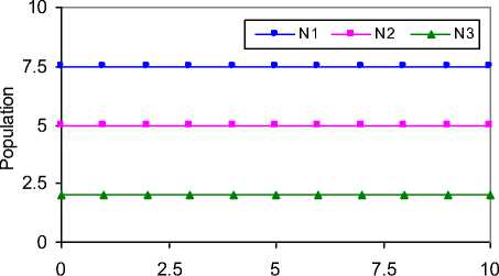
The numerical solutions of the discrete model equations computed for specific values of the various parameters and the initial conditions. The results are illustrated in Figures 1 to 6.

N ( t ) = n ( t + 1) = n ( t + 2) =...........

a ₁₁

^{( a} 1    1 ) ^{+ a} 12 a 23

(      1A a -1

V a 22 a 33 J

⁺ a 13

a - 1

V a 33   J

N ( t ) = N ( t + 1) = N ( t + 2) =

= a 23

a - 1

V a 22 a 33

N ( t ) = N ( t + 1) = N ( t + 2) =

a^ — 1

i.e, N j ( t + г ) = — a 11

I a - 1 1     I a - 1

^{( a} 1 ^- 1 ) ⁺ a ₁₂ a 23 I           I + ^a 13 I

V a 22 a 33 J      V a 33

I a - 1

N ₂ ( t + г ) = a ₂₃ I -------

V a22 a33 J where r is an integer Hence, E13 is stable.

a - 1

, N3 (t + Г) =  - a33

N. Stability of E 14

N ( t ) = N ( t +1) = N ( t + 2) =...........

^a 11

a 12 a 23

(, a

-1 ^

V a 22 a 33 J

^{+ a} 13

a -1

V a 33 J

N ( t ) = N ( t + 1) = N ( t + 2) =

I a - 1 = a ^{23 1}

V a 22 a 33

N ( t ) = N ( t + 1) = N ( t + 2) =

a - 1

N ( t + Г ) = — a ₁₁

N ₂ ( t + г ) = a₂₃

a -1

⁺ a 13

a -1 ^

V ^a 33 J.

a 12 a 23

V a 22 a 33

V ^a 22 a 33 J

, N ₃( t + Г )

a -1

a ₃₃

where r is an integer Hence, E₁₄ is stable.

At this stage all the fourteen equilibrium states are stable.

• Two period equilibrium states (Stage-II)

N i ( t + 2) = N i ( t ), i = 1,2,3

Time

Fig.1. Variation of population against time for α 1 =3.9, α 2 =2.6, α 3 =4.4, a 11 =1.18, a 12 =0.6, a 13 =1.5, a 22 =0.8, a 23 =1.2, a 33 =1.7, N 10 =7.5, N 20 =5, N 30 =2

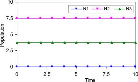
Fig.2. Variation of population against time for α 2 =1,

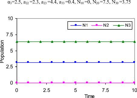
Fig.3. Variation of population against time for α2 =1, α3 =4.2, a11 =3.2, a13 =1.6, a33 =0.5, N10 =3.2, N20 =0, N30 =6.4

(One Period Equilibrium States)

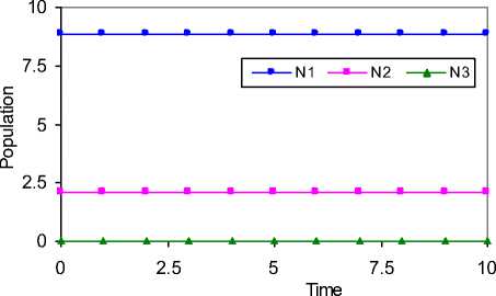
Fig.4 Variation of population against time for α2 =1, α2 =2.7, a11 =1.4, a12 =5.85, a22 =0.8, N10 =8.9, N20 =2.1, N30 =0

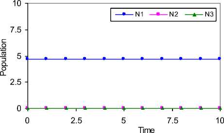
Fig.5. Variation of population against time for α1=3.8, a11 =0.6, N10 =4.7, N20 =0, N30 =0

Fig.6. Variation of population against time for N10 =0, N20 =0, N30 =0

• VI.    Conclusion

The present paper deals with an investigation on a discrete model of three species syn eco-system with limited resources. The basic equations for this model constitute as three first order non-linear coupled ordinary difference equations. All possible equilibrium points of the model are identified at N ( t + 1 ) = N ( t ) ; i = 1,2,3 . It is observe that, all the fourteen equilibrium points are found to be stable. Further the numerical solutions for the discrete model equations are computed.

Acknowledgment

I thank to Professor (Retired), N.Ch. Pattabhi Ramacharyulu, Department of Mathematics, National Institute of Technology, Warangal (A.P.), India for his valuable suggestions and encouragement.