A Survey of Compressive Sensing Based Greedy Pursuit Reconstruction Algorithms

Published Online September 2015 in MECS

Reconstruction is an inverse problem in which an image or signal can be recovered from the data given. The given data can be in the form of codes, from which data samples are required to be acquired and processed in order to recover the image or signal accurately. In this paper, the various techniques for image reconstruction using Compressive Sensing are discussed. Compressive Sensing is a highly efficient technique because of the high need for rapid, efficient and less expensive signal processing applications. Earlier, signal processing techniques employed Nyquist-Shannon theorem. This technique requires sampling rate to be at least two times the highest frequency in the signal. This requirement for the sampling frequency is called Nyquist condition. This theorem finds applications in many audio electronics, medical imaging devices, visual electronics, radio transmitters and receivers [1]. However, this technique requires larger storage space, running time and computations. Moreover, in some of the processes, there may be the only limited number of samples available or may be only limited data capturing devices or slow measurements. In such situation, Nyquist-Shannon theorem fails and Compressive Sensing (CS) is able to use the concept of sparsity using different transform domains and incoherent nature of these observations in the original domain. CS offers sampling and signal compression in one step and measures the only minimum number of samples that can carry the maximum set of information [2]. CS is one of the novel techniques that do not require the Nyquist sampling rate for image processing. The implementation of CS reduces the requirement of acquiring and preserving the large number of samples. It saves only those samples, which have significant value and samples with minimal value are discarded. CS offers various applications due to its property of sparsity and incoherence. This paper presents a brief historical description of CS and analyzes the various CS based image reconstruction algorithms. In this paper, section I presents the introduction of Compressive Sensing and image reconstruction. In Section II, background and implementation of Compressive Sensing are discussed with certain properties. The Section III presents ℒ2_ minimization recovery algorithm. Section IV presents Matching Pursuit, Orthogonal Matching Pursuit (OMP) and its latter modification Regularized OMP (ROMP). In Section V, the working of Iterative Hard Thresholding algorithms is discussed. In the Section VI Generalized OMP (GOMP) and Adaptive GOMP (GOAMP) are presented. The discussion and analysis is presented in Section VII. The paper is concluded in Section VIII.

• II.    Compressive Sensing and Background

In engineering theory and practical applications, the sampling theorem of Nyquist-Shannon theorem has a tremendous role but it can be used frequently only for band-limited signals otherwise it requires larger storage space and measurements for high-dimensional signals. However, practically reconstruction is even possible with fewer measurements and compression is also needed before storage. These requirements can be fulfilled with

Compressive Sensing. The field of CS has gained enormous interest recently. It is basically developed by D. Donoho [3], E. Candes and T. Tao [4]. It was used in Seismology for the first time in 1970 and then later on ℓ2_ norm minimization was suggested by Santosa and Symes for recovery algorithms [5]. Then, total variation minimization was used by Ruden, Fatemi and Osher [6] in 1990s for image processing. The implementation of total variation minimization is somewhere identical to ℓ-£ norm minimization. But, the idea of CS was actually taken into account by D. Donoho, E. Candes, Justin Romberg and T. Tao [3, 4].

• A.    Nyquist Sampling Theorem

  Shannon proposed his famous Nyquist-Shannon Theorem in 1949. According to Shannon theorem, any band-limited signal, time varying in nature can be recovered perfectly if the sampling frequency is numerically equal to or greater than two times of the maximum frequency present in the signal itself. For a signal of frequency И Hertz, sampling rate requires to be 1/2и seconds. For conventional processes, before transmission of the data or signal, it is sampled properly at Nyquist rate followed by compression. For example, if the data is sampled at и hertz and then compressed to 'S' samples and и-S samples are discarded. At the recovery part, for most decompression is performed and 'и ' samples are extracted from compressed ' S ' data samples. In Fig. 1, x is the signal of interest and y is the compressed measurement vector. The figure depicts a model of Traditional Sampling Technique, in which acquisition and sampling are separate steps. In this approach, the number of captured samples remains greater than the information rate. This technique is computationally complex, especially for the highdimensional signals, due to the requirement of the large storage space. Moreover, analog to digital conversion for high dimensional signals is expensive. The question that arises after studying the Nyquist-Shannon Theorem is that what is the need of overall computation when only 'S' data samples are sufficient.

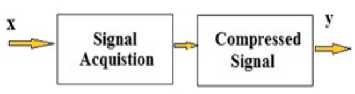
Fig.1. Structure of Traditional Sampling Technique

Compressive Sensing ‘

Model (Compression + Sampling )

• Fig.2. Structure of Compressive Sensing paradigm

The compressed form contains major information; hence there is no need of computing rest of the nonsignificant samples. So Compressive Sensing is an alternative approach, which performs sampling and compression together as shown in Fig. 2.

• B.    Compressive Sensing

CS theory enables the implementation of the recovery of the high dimensional signal from lesser observations as a comparison to the actual number of measurements required in conventional techniques. The objective of CS recovery algorithms is to provide an estimate of the original signal from the captured measurements. It is based on the property of the signals to be able to offer their representation in the sparse domain with fewer numbers of nonzero coefficients. This property is called sparsity and the given signals as sparse signals. The reconstruction algorithm used with CS decides the number of samples needed for exact reconstruction. The model of reconstruction using CS depends on two properties:

• 1)    Sparsity

Many signals are capable to be stored in compressed form in terms of their projection in a suitable basis. The projected coefficients of these signals can be zero or a far lower value, if a suitable basis is used. For a signal having к non-zero coefficients, it is called к -sparse. As, these sparse signals may offer the larger number of smaller coefficients that can be ignored easily; hence a compressed signal can be obtained from the sparse form. For compressive Sensing, the suitable domains available are DCT, DWT, and Fourier Transform [7]. Discrete Wavelet Transform is usually preferred over Discrete Cosine Transform because it enables the removal of blocking artifacts [8]. Basically, Sparsity refers to the possibility of having a much smaller information rate for a continuous time signal as a comparison to the one depicted by its bandwidth. So, CS can use the advantage of using these natural signals with their compressed form in a particular domain. Suppose a signal х can be represented in a suitable orthonormal basis like wavelet, DCT. As in a signal, many coefficients are small and most of the important information lies in few larger coefficients. Hence, it can be expanded in an orthonormal basis for sparse representation. Let х the given signal and ф ={ Ф1 ……… •фп } represents the suitable basis, therefore, an image X in domain ф is given as:

X (t)=∑ 'Uwtipt ( t ) (1)

where w is the coefficients of the sparse form of X , W[ =‹ X , ф[ › . In a sparse representation of the signal, small coefficients in that signal can be neglected without much information loss. It's like considering the signal X by keeping only the significant coefficients and discarding the smaller coefficients. Thus, the obtained vector is known as a sparse signal.

• 2)    Incoherence

Incoherence shows that any signal with a sparse representation in a particular domain can be spread out in a domain in which it is actually captured. It enables the relationship of duality between time and frequency. It measures the maximum correlation for any two matrices. These two matrices give a form of different representation domains. For the measurement matrix Φ with м×N size and the representation matrix Ψ of N×N size, the representation matrix can be represented as ѰL……․․Ѱ as columns and measurement matrix as Φ 1 ………Φ as rows. The coherenceЦ is given as:

ц (Φ,Ѱ)=√ nmax |Φ к Ѱ |         (2)

for 1≤ j ≤ n and 1≤ к ≤ m . Moreover, from linear algebra, for incoherence following result can be depicted:

1≤ Ц (Φ,Ѱ)≤√ n           (3)

In CS technology, the incoherence of two matrices is important. One is the Sensing matrix that is used to sense the significant columns of the signal of interest. The second one is the representation matrix Ѱ in which the given signal is represented in the sparse form. The low value of incoherence for CS shows that the fewer measurements are required for reconstruction of the signal [9]. Coherence is able to measure the maximum correlation between the columns or elements of Φand Ф . Mostly low coherence pairs are considered in Compressive Sensing. The measurement matrix Φ basically performs the function of sampling the coefficients. The measurement matrices like Fourier, Gaussian are able to satisfy the coherence property. The random matrices like i.i.d Gaussian Matrix or binary ±1 matrix with fixed basis Ф are mainly incoherent. These matrices are simple and possess lower convergence, which are required for recovery with Compressive Sensing.

• 3)    Restricted Isometry property (RIP)

RIP is one of the most important properties of Compressive Sensing. It can be used as a tool in order to analyze the performance implementation of CS. RIP tool is able to ensure that the sensing matrix captures the significant columns from the given signal of interest. This property can give the condition for the reconstruction matrix for exact recovery. For any К sparse signal v , restricted isometric constant (RIC) 6_K (0< Sr <1) is the minimum value that makes the inequality holds [10]:

• _(1- 5k )‖ v ‖ X ≤‖ΦV‖ X ≤(1+ 5k )‖ v ‖ X     (4)

When this property holds, then the matrix 6 can preserve the Euclidean length of К-sparse signals, which shows that the given sparse vectors are not in the null space. It can be considered as the sufficient condition for recovering the estimate of the support for the sparse signal. If RIC constant is not really close to 1, then the property ensures that all the columns selected are orthogonal and the sparse signal is not in the neglected part of the matrix which is sensed. Otherwise, it cannot be reconstructed. For the relation of CS and RIP property, it is shown that if К -sparse signals are required to be recovered, then 6К should be lesser than 1. This ensures the recovery of sparse signals from observations vectors with compressive Sensing. The restricted isometry property can be considered as the form of uniform uncertainty principle for many ensembles of random matrices like Fourier, Gaussian, and Bernoulli [4, 11]. These matrices satisfy the RIP condition with parameters 6 € (0,1/2) which can be represented by Eq. (5).

M =       ⁽¹⁾ N                 (5)

where M is the number of measurements and N be the dimension of the signal, К is the sparsity of the signal. Therefore, a signal can be recovered exactly for M measurements, К is the sparsity. In some applications, measurement matrices play an important role. Some of the measurement matrices include Fourier matrix having randomly selected rows. The complexity, in this case, can be reduced by using Fast Fourier transform. Bernoulli matrix which can also be used as measurement matrix has faster Sensing but storage complexity. The Gaussian random matrix is another measurement matrix which is derived from the normal distribution with zero mean and variance 1/N. Gaussian matrices are very simple and useful operators for Compressive Sensing. Gaussian matrix is mostly preferred because of its simplicity and easy implementation.

• 4)    Compressive Sensing Model

Compressive Sensing model basically performs compression and sampling simultaneously. Considering an N -dimensional signal x , the sparse form of the signal can be constructed by representing it in any suitable basis like DCT, Fourier Transform, and wavelet Transform. The sparse form or the signal of interest can be given as:

w=                      (6)

where w is the sparse form of X and "Ф is the suitable basis that shows the projection coefficients of w on the given basis. The next step is to compute the measurement vector у with a suitable matrix either Gaussian [12] or Bernoulli [13]. The measured vector can be given as:

У=Φи/                (7)

where Φ is the measurement matrix of dimension м × N . The overall Eq. can be represented as:

У =Θ х                (8)

where Θ is the Sensing matrix and is depicted as Θ=Φ "ф , it is also known as reconstruction matrix. In practical applications, the measurement or the random noises can also be considered. Equations (6) and (7) are reformulated as:

У =Φи/ + 9             (9)

У =Θ х + 9             (10)

where 9 represents random noise vector. Hence, the primary objective of CS is to recover the signal from these captured measurements, under sparsifying conditions. Then, the recovery algorithms are applied on the given measurement vector. The recovery algorithms available are ℒ 1 minimization, several Greedy algorithms which are discussed in the next section.

• III.    ℒ! Minimization

For recovering the sparse signal from its observed measurements, recovery algorithms are required. Convex relaxation is the class of algorithms which can solve reconstruction issues through linear programming [14]. The number of measurements needed for these techniques is small, but the methods are complex in computational terms. The recovery problem needs to solve the highly convex problem according to (11).

min ‖ X ‖Q subject to у=Φ X (11)

It was later suggested by Donoho and his associates that for given measurement matrix, ℓо as an NP- hard problem can be considered equivalent to its convex relaxation i.e. ℓ 1 minimization.

min ‖ х ‖ 1 subject to у=Φ X (12)

where ‖ X ‖ = ∑ I | Х( | denotes the ℓ - norm. This kind of convex reconstruction problem can be solved by linear programming. For ℓ minimization, the measurement matrix must satisfy RIP property for a small value of Restricted isometric constant (RIC). BP (basis pursuit) [15], BP de-noising are some of the examples of ℓ 1 minimization techniques. It allows the recovery of norm minimization instead of recovering the low-rank matrix from the compressed form of the signal. This algorithm reduces the complexity, dimensions and order of the system because low-rank matrix signifies low order and less complex system. Basis pursuit works as an optimization problem and minimizes the cost function constructed by the Lagrange multipliers.

min(‖У-Φ т ̌‖2+Л‖ ̌‖1 (13)

where л is a positive constant. The algorithm works in simple steps by first initializing the sparse signal and providing the cost function. The Sensing matrix is computed by selecting the required number of measurements and then the coefficients of the sparse image are modified in order to obtain the minimized form. The iterations work until the number of total significant components remains less than к , sparsity of the signal.

• IV.    Orthogonal Matching Pursuit (OMP)

The greedy algorithms are iterative approaches; capable of recovering the images using Compressive Sensing. Block based Compressive Sensing enables the use of Greedy algorithms for recovering thermal images also [16]. It works in an iterative fashion in order to recover the sparse signal. Orthogonal matching pursuit (OMP), a greedy algorithm, basically comes into account in the form of a variant of MP (Matching Pursuit) algorithm. Earlier, the MP algorithm, an iterative greedy method, was introduced in order to approximate the decomposition [17]. It identifies those bases and their coefficients; that can construct the input signal on combining. It starts with the assumption that all the bases are orthogonal to each other i.e. independent of each other. The value calculated by correlation of the given signal with the basis gives the influence of basis on the signal. For the basis to be the important part of the signal; correlation value should be high and for a lower value of the correlation, the basis has a negligible contribution. It works by selecting the elements having the maximum correlation with the residual vector throughout the algorithm at each step.

Let ф₍ 1< i < N , be the element having the strongest correlation with residual г , denoting the it ℎ element of measurement matrix Φ . All atoms are assumed to be normalized with value unity. The selection of elements by the algorithm, at each iteration, is represented as:

Фк = |‹ ^гк-1 , Ф[ ›| (14)

where the inner product is denoted by ‹.› and ^*1^—3^ shows the residual at к -1 iteration.The algorithm then updates the residual depending on the column selected till the termination criterion occurs. When the halting condition occurs, the algorithm stops i.e. when the value of the norm of residual becomes lesser than the predefined threshold or error bound. The algorithm may stops even when the number of distinctly selected elements in the approximation set becomes equal to the desired limit. The Matching Pursuit algorithm is used mostly because of its simplicity. But it suffers from the drawback of slow convergence and poor sparse results.

The orthogonal matching pursuit (OMP) [17, 18] has the capability to remove this drawback by projecting orthogonally the signal on the subspace corresponding to the selected set of columns. The method of selecting the elements remains the same in both the algorithm. As OMP is based on orthogonalization, an atom is selected only once throughout the algorithm. Y. C. Pati et al., demonstrated OMP as the recursive algorithm, to calculate the functions in the form of the non-orthogonal basis using wavelet frames.

OMP constructs the orthogonal projection onto the observation vector. Before the orthogonal projection, the algorithm computes the inner product of the residue and the measurement matrix. Then the coordinate of the highest magnitude is selected and the column corresponding to that coordinate is extracted. These columns are then embedded into the selected set. It offers better asymptotic convergence as comparison to the conventional MP algorithm. OMP algorithm is considered as a powerful and fast recovery algorithm for the sparse signal from the random measurements. It can provide recovery results for M measurements and N dimension with О(MlnN) random measurements. It is a huge improvement over the conventional recovery algorithms. OMP algorithm has an evident place because of its speed and easier implementation. Consider a given signal X of dimension N. Select the number of measurements required i.e. M. Construct measurement matrix Φ of dimension M x N. Then, obtain the sparse form of the signal X and construct the observation vector У=Φх, this measurement vector is of dimension M, hence obtaining the compression and sampling in one step. OMP algorithm works step by step. The OMP algorithm searches for the significant column in the inner product of the residue and the measurement matrix. Then, the orthogonal projection is computed onto the subspace of the measurement vector. This orthogonal projection gives the estimate of the support set. The residue is updated according as the estimate. The iterations continued until the residue is lesser than the specified threshold. Finally, the recovered signal is obtained in terms of the estimate of the support system. For the termination of the algorithm, the norm of the residue can be checked with respect to the threshold. Here, the residual rt is always orthogonal to the columns of the measurement matrix. The conditions for termination of the algorithm can be based on cumulative coherence property [19]. This algorithm selects a new significant column at each step. The column selected corresponds to the index having maximum inner-product. Then, this selected column is augmented with the initialized set. The residual is updated with each step for the new estimate of the support set. Finally, the estimate of the sparse signal is computed with the updated residual. The running time of the algorithm is depicted by the step of identifying the new indices. A prototype of OMP algorithm first came into account in 1950 [20, 21]; later on it was investigated further for its implementation in recovering the sparse image from random measurements with noise in year 2011 by T. Tony Cai and Lie Wang [22]. The OMP algorithm was studied with bounded noise and its recovery performance is checked under such condition. The implementation of OMP provides an effective way of recovering the sparse signal from random observations even in the presence of noise with appropriate measurement matrix. The steps of the OMP algorithm are given as follows:

OMP Algorithm

• •    Initialize the index set ∧ _к= ∅ and the residue r₀ = and the counter set t=1

• •    Identify the coordinate for which the inner-product is highest

∧ t =              …․ |‹ r_t-l ,Φ i ›|

• •    Take the selected index set and augment it with the matrix of chosen atoms ∧ £ = ∧ t— 1 ∪ { ∧ £} .

• •    Compute the least square problem in order to obtain the new estimate of the sparse signal:

X_t =       ‖ У -Φ _tX ‖ 2

• •    Estimate the newly updated approximation of the residue:

«t =Φ _tx_t П =  ^- «t

• •    Increase the counter number and go back to step 2 if t < K.

• •    The value of the calculated estimate gives the recovered signal.

Later on, Subspace Pursuit (SP) is suggested, which considers multiple indices at each step and keeps only K coefficients for the support set throughout the algorithm [23]. SP algorithm is able to provide low computational complexity with a comparable capability for every sparse signal. The algorithm can be used for both noisy and noiseless observations. It can reconstruct the К -sparse signal accurately from noise-free observations when the sensing matrix 6 satisfies the RIP property. For the inaccurate measurements, the distortion is limited by the constant which is a multiple of measurements. The basic idea of the SP algorithm is extracted from coding theory. Here, the set of к columns representing the information are selected. These symbols have the maximum correlation. Their selection is basically a hard-decision, thus, metric for the parity checks are computed. The other lower coefficients in these selected atoms can be adaptively changed in a sequential order on the basis of this metric. At iteration t, the algorithm selects K indices with the largest magnitude of the inner-product: Φ T_rt-i . By selecting these coefficients, the support set is expanded. Then, an orthogonal projection is computed for the selected support set by taking the estimate of y onto the measurement matrix, corresponding to the selected indices. The iterations work until residue falls below the certain limit. Subspace Pursuit is capable of providing simple implementation and accurate results.

On the other hand, the approach of CoSaMP is based on restricted isometry property. The restricted isometric constant of measurement matrix Φ is considered lesser than 1. Then, for the К -sparse signal x , having a vector У =Φ ∗ Φ x can be considered as an equivalent representation of x . This is due to the fact that the energy in К components of У is equivalent to the energy in the к components of х . Hence, the highest atoms of х can be represented by the highest atoms of У . Hence, the recovery of sparse signals becomes easier. CoSaMP expands the support set by 2K elements. Then, the orthogonal projection is computed taking y onto Φ _t at each iteration corresponding to K indices. The process terminates with the stopping condition ‖ г new ‖ 2 ≥‖ г ‖ ₂. These algorithms reduce the reconstruction error when certain RIP condition occurs [24]. These algorithms use a fixed size of the support set and the knowledge of a priori estimate of sparsity K is necessary. This is a major drawback in practical cases where K is either unknown or it is not fixed.

The OMP algorithm was later modified with the regularization step. The regularized OMP is able to recover the sparse signal from random measurements within considerably reduced time interval. Deanna Needell and Roman Vershynin proposed ROMP for sparse recovery which gives the advantage of fastest implementation [25]. The regularized OMP performs accurately the recovery for all measurements matrices under RIP conditions for all kind of sparse recovery. It starts with sparsifying the given signal of dimension N with measurement matrix Φ . Then, the measurement vector is constructed У=Φх . This measurement vector is operated on in order to recover the signal. The algorithm selects the S largest coefficients of the inner-product rather than identifying the only the largest one. Thus by considering multiple indices at a time and then considering only those having energy greater than a particular threshold, total running time can be reduced considerably.

The ROMP algorithm works until the iteration count becomes greater than twice the Sparsity value, K. The ROMP algorithm is able to prove the stability bound without the logarithmic factor. Even, it does not need the prior knowledge of the given threshold or tolerable error. The running time of ROMP is very less as compared to the OMP algorithm. The identification of the multiple significant columns in ROMP is based on the regularization step. This step requires considerably low time. In a ROMP technique, the first step is to select the number of measurements м . A residual, index set are considered as: т₀ = У , ∧ Q = ∅ , where y is the measurement vector. The algorithm selects the set / of the 5 highest non-zero components having the maximum magnitude of the inner product Φ T_rt-i , for all coordinates. Then, the step of regularization comes in which among these sets, set J 0 is taken into account, which a subset of / for having maximal energy is. These selected coordinates in the set are then added to the initialized index set. The residual is updated for each time the set is augmented. The algorithm halts when the stopping condition meets i.e. until | ∧ | ≥ 25 , where 5 is the predefined size for the selection of atoms at each iteration.

• V. Iterative Hard Thresholding Technique

The Iterative Hard Thresholding (IHT) algorithm for the first time was suggested by Blumensath and Davies for recovery in compressed Sensing scenario [26]. This algorithm can offer the theoretical guarantee with its implementation which can be shown in the particular one

• [27]. The basic idea of IHT is to chase a good candidate for the  estimate of support set which fits the

measurement. The iterative hard thresholding (IHT) algorithm is an algorithm with a simple implementation. It requires the application of the operators corresponding to the measurement matrix i.e. Φand Φ т . Both operators are required once in each iteration, with the operation of two vector additions. The partial ordering of the elements of ^t =   +ΦT(У-Φx^) in magnitude requires the operator Hs . The implementation of IHT requires lesser storage. The algorithm requires the storage of the measurement vector У and the sparse signal. The operators Φ and Φт may create the computational complexity in terms of running time and storage. If the measurement matrices are the general matrices, then the computational complexity reduces considerably. The common operators which are based on Fourier Transform, Wavelet Transform are used for the higher dimensional problem, which leads to the reduce requirement of memory. Suppose Xo = 0 and use the following iteration step:

^t+l = ( ^xt +Φ T ( У -Φ ^xt ) (15)

where H_s (w) is the non-linear operator that sets all the S largest elements of w to zero. A set can be selected randomly or in terms of any previously defined order of the elements if no such unique set exists. In this case, the above algorithm converges to a local minimum of the optimization problem.

т1тг_х ‖ У -Φ x ‖2 (16)

Iterative Hard Thresholding is a technique that provides accurate recovery results from sparse measurements with the optimization problem. IHT is the class of algorithms that offers guarantees for near optimal error. Its performance remains robust even in the presence of noise. This algorithm can perform well with lesser number of measurements. The memory requirement depends on the size of the problem. The computational complexity is lower, depending on the number of captured observations. The fixed number of iterations is required by the algorithm depending on the signal to noise ratio. The iterative Hard Thresholding can be implemented in two forms as Fast IHT (FIHT) and Forward- Backward Pursuit (FBP). Fast Iterative Hard Thresholding was suggested as a variant of Algebraic pursuit, though it uses a support set by taking other indices with respect to the large candidates of the residual of particular cardinality.

However, Algebraic pursuit uses larger support and extracts the correct and significant support of the observed vector, FIHT uses smaller size support set in order to more accurately reducing the residue. It is a special case when the support is correctly located. FIHT has better convergence and performance than algebraic pursuit [28]. Forward Backward Pursuit is also one of the iterative hard thresholding algorithms. This algorithm uses two stages: forward stage and backward stage. The forward stage includes the addition of the selected indices and the backward stage includes removal of the nonsignificant columns. This movement expands the support set and shrinks it simultaneously in an iterative manner. This algorithm is an iterative hard thresholding that uses the concept of expanding the support iteratively. The major advantage of the FBP is that it does not require the knowledge of sparsity К in advance. In most of the scenarios, FBP is able to perform better than SP, OMP, and BP.

In this algorithm, after implementing compressive Sensing on the given signal FBP is applied. In the forward step, the algorithm identifies the a indices corresponding to the maximum magnitude of the inner-product of residual and the measurements. In this step, the forward step size a should be greater than 1. Next, the orthogonal projection is computed for the columns corresponding to the selected a indices. Then, backward step is applied by cropping the support set estimate. It removes p indices from the estimate of the support set which are the indices having the minimum magnitude of the orthogonal projection. In this algorithm, the final orthogonal projection is computed for the columns corresponding to the cropped set. For the successful recovery of the sparse signal using FBP, it is required that a>P . Thus, the number of indices added should always be greater than the number of indices removed [29].

The steps or the implementation of FBP algorithm can be as shown as follows:

Algorithm of FBP

Initialize: ?о = ∅ , r° =  , к =0

• •    while true do

к = +1

• •    = {indices corresponding to a maximum magnitude

coefficients in Φ T_r ⁽ k-1⁾}

̌ ⁽ к )₌ s ⁽ k-1 ) _∪ T_f

̌ = argmin ‖ У - Φ ̌ ( к ) ̌‖

• •    T_b = {indices corresponding to p minimum magnitude coefficients in ̌ }

s ⁽ к ⁾ = ̌ ⁽ к )_- Ть

• •    Projection: w =        ‖ У -Φ_s ( к ) ̌‖

• •    Residue update:Г⁽ к ) = У -Φ_s ( к ) W

• •    Termination rule: Algorithm works until

‖ _rk+l ‖2≤E‖ У ‖ г and | _Tk |≥ ^max .

• •    Outputs: S^(k), x_s ( к ) =ΦJ ( к ) У

The FBP algorithm uses the threshold parameter г in order to check that the current residue is within the range. Its value depends on the level of noise present in the given signal for noisy observations. In this case, there is no requirement of sparsity К , but the iterations can be limited with the parameter ^max . For the accurate performance of FBP, it is require having the forward parameter greater than the backward parameter so that a suitable range of support set is selected at each iteration [30]. The а can be considered as [0.2 М , 0.3 М ] and р < а - 1 for the faster implementation of the algorithm. FBP usually succeeds in the majority of cases but the failure may begin when ^тах > 55. It is easy to implement the algorithm that can expand support set iteratively and recover the sparse signal precisely.

VI. Generalized OMP

Generalized OMP (GOMP) is basically a clear generalization of the OMP algorithm. It selects multiple indices rather than identifying only one as in the case of OMP algorithm. As multiple indices are selected at each iteration, hence lesser numbers of the iteration are required for overall recovery. It provides exact recovery for К -sparse si g nal where the restricted isometric constant 6_К <  ^√   . Generalized OMP is basically an

√ к+з√.                              y extension of OMP algorithm with better efficiency and recovery probability. In each iteration step, GOMP computes the correlation of the columns of measurement matrix Φ and the residual. Then, these correlations are compared and the indices corresponding to the S maximum correlation are selected. The support set is extended using these S indices and the least mean square problem is solved. After this, the residue is updated by eliminating the orthogonal projection from the measured vector [31]. This orthogonal projection corresponds to the indices with maximal correlation. These steps are repeated until the iteration count reaches its maximum set value. This algorithm provides better recovery results within reduced running time as compared to the already existing algorithms. For GOMP algorithm, the complexity of the overall algorithm is О(MN) where M is the number of measurements and N be the dimension of the given signal. The threshold parameter specified in this algorithm is used to check the magnitude of the residue so that it remains within the range. GOMP is potentially more effective than OMP algorithm in recovering the sparse signal from random measurements within a specified time interval. Hence, we can say that the convergence speed of GOMP algorithm is better than OMP. The steps for GOMP algorithm are as shown:

GOMP algorithm

Initialize: The index set ∧ _к= ∅ and the residue г₀ = and the counter set t=1.

Steps:

• •    while ‖  ‖ ₂> г and к < min{ К , М / N }

к = +1

• •    Identify indices corresponding to the S largest entries in Φ T_rt-1 in magnitude.

• •    Augment the selected indices with the existing support set

∧ t = ∧ t-1 ∪ {Φ(1)……․Φ(5)}

• •    Calculate the estimate for the sparse signal

̌_t=        ‖ У -Φ _tw ‖ 2 (24)

• •    Update the residue according as the estimate: T_t =  -Φ t ̌ t

End

• •    Provide the Output: ̌£ =        ‖ y_ -Φ _tw ‖ 2

Later, GOMP algorithm was made adaptive in order to eliminate the need of sparsity before the algorithm. Basically, value S i.e. the number of indices selected at each iteration defines the actual performance of the algorithm. Generalized Adaptive OMP makes this value, S, adaptive through the iterations as the residue reduces. As the columns identified initially have a greater role to play hence an optimal value of ‘S’ is required. This ensures that any wrong atom is not selected. Further, the factor ‘S’ keeps on incrementing depending on the reduction in the residue. The Generalized adaptive OMP has rapid convergence and moreover there is no need of sparsity [32]. The number of columns selected increases at each iteration with a decrease in the residual through the algorithm. In GOAMP algorithm, J indices are selected for having the highest magnitude in the correlation of measurement matrix and the residue. These J indices are then augmented or added to the initialized index set. The residual is updated for the new orthogonal projection of the measurement matrix onto the measurement vector corresponding to the new coordinates. Then the size of selecting atoms increases if the residual decreases through the algorithm. So, through the algorithm the step size increments so that the atoms are selected adaptively. The algorithm works until the residual falls below the specified threshold. Finally, the residual is updated and the recovered signal is obtained. The GOAMP algorithm uses two thresholds. Usually, the value of thresholds depends on the value of noise available in the given signal for measurements in the noisy environment. Otherwise, the thresholds are selected considering the number of atoms to be selected at each iteration. The GOAMP algorithm provides exact recovery with not having the knowledge of sparsity K. It provides acceptable results even in the presence of noise. This algorithm provides the mean to identify the significant column and then increasing the size of the number of the column selected adaptively on the basis of the decrement in a residue. Hence, it is able to provide suitable results for recovery from sparse observations.

• VII.    Discussion and Analysis

The concept of image reconstruction with compressive Sensing is not only a useful combination for image recovery, but also comes with its ease of implementation. The CS based image reconstruction algorithms include Greedy pursuit algorithms and convex minimization methods. These algorithms can be implemented in the field of communication, medical images, signal processing and networking systems. Due to faster, cheaper and efficient implementation of CS-based image reconstruction; it has larger perspectives. The greedy algorithms even provide reconstruction on the basis of orthogonal projection for the selection of significant columns only. The greedy algorithms work in an iterative fashion. It works in a step by step fashion in order to recover the images from random measurements. One of its algorithms i.e. Matching Pursuit is able to overcome the drawbacks of 1г minimization. Although, due to slower convergence, it was later replaced by Orthogonal Matching Pursuit; it provides the selection of orthogonal columns with highest correlation so that each atom selected is unique. It is preferred mostly because of its simplicity.

The termination conditions for OMP can be based on coherence, cumulative coherence, RIP; it can be further optimized in order to ensure the selection of significant components only. The ROMP was later introduced in order to reduce the overall running time by selecting multiple indices. The Generalized version of OMP helps in recovering the images or signals accurately with multiples indices at each iteration. The Generalized algorithm was later made adaptive in order to select the size of atoms selection set according as the decrement in the residue. Earlier, the knowledge of sparsity was required but the adaptive algorithm eliminates this requirement. Table 1 compares the recovery performance of the greedy pursuit algorithms for the reconstruction of the image. The recovery performance is analyzed in the form of PSNR value obtained and running time elapsed. It shows the PSNR value and running time elapsed for the implementation of these algorithms and provides comparative results in a tabulated form.

Table 1. Comparison of Recovery Performance of Different Techniques

Recovery performance parameters for M=128	PSNR (dB)	Time (sec)	Complexity of the algorithm
Subspace Pursuit	25.76	52.38	0 (KMN)
Orthogonal Matching Pursuit	25.01	8.54	о (км n
Regularized OMP	21.84	2.31	о (км n
Generalized OMP	27.82	8.63	0 (MN)
Generalized adaptive OMP	28.82	4.52	0 (MN)

(a)

(b)

(c)

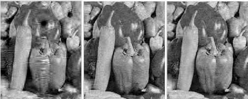
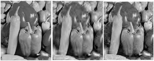
Fig.3. Comparison of Reconstruction Results for M/N=0.5 (a) Original Image (b) SP Method (c) OMP Method (d) ROMP Method (e)GOMP Method (f) GOAMP Method

In Fig. 3, the recovery performance of greedy algorithms has been demonstrated in terms of visual outcome. The simulation is done on standard grayscale 256 x 256 'peppers' image. The result of greedy pursuit algorithms is shown for the sampling ratio M/N=0.5. The conventional CS measurement matrix i.e. independent and identically distributed Gaussian matrix with mean zero and standard deviation 1/N is used. All simulations are performed in MATLAB 7.6.0.The experiments are run on a laptop with Intel core i5 CPU at 2.5 GHz and 6 GB under windows 7. In Fig. 3, the recovery results of the greedy pursuit reconstruction algorithms are demonstrated. It provides the comparative analysis of the reconstructed result for each algorithm. The visual quality of recovered image is better in case of Generalized OMP which is able to secure the fine details of the given image.

The implementation of CS-based reconstruction to exploit the sparsity in 3D video frames can be used for 3D video coding, and recovery and communication on mobile hand-held devices in future. The medical MRI and CT images can also be recovered efficiently with lesser storage requirements. The photo-acoustic images and the recovery of the satellite captured images, images for remote sensing can easily employ CS based recovery; thus providing only the storage of fewer components and saving the memory or database. The Compressive Sensing based image reconstruction can be used in RADAR imaging, biomedical imaging, and mobile communication. The reconstruction based on Compressive Sensing can be implemented for color images and in digital cameras. For the suitable basis, the multistage sparse representation can be adopted for better accuracy.

In future research, the bounds can be tightened more. These bounds are concerning the termination conditions in the recovery algorithms. The sparse correlation bound can be used for recovering and the algorithm for speed up can be considered. The Generalized OMP can be made more effective by using improved probabilistic analysis. The Generalized Adaptive technique can further be optimized for its implementation with noisy images. The Basic advantage of the CS based reconstruction with these algorithms includes faster and easier implementation, fewer storage requirements, lower computational complexity and wider scope of their implementation in different fields.

• VIII.    Conclusion

In this paper, Compressive Sensing paradigm and the Compressive Sensing based image reconstruction algorithms are analyzed. Various recovery algorithms like ℒ 1 minimization, Basis pursuit, Subspace pursuit, OMP, GOMP, ROMP, IHT and their variants have been considered. The reconstruction algorithm uses the process of sampling the components which tend to require larger storage space, which is largely reduced by compressive Sensing techniques. Compressive Sensing based reconstruction algorithms uses lesser number of data samples, provides faster computation, and lesser memory requirements. Thus, it eliminates shortcomings of conventional sampling techniques. In this paper, computational complexities along with the running time of these recovery algorithms have been compared. The OMP method offers simple and faster recovery as comparison to the Matching pursuit method. Though, the performance for generalized algorithms is better than OMP. The PSNR value is better for GOAMP as the comparison to the other techniques.

On the contrary, ROMP technique provides considerably shorter running time but the visual quality lacks considerably than the generalized algorithms. For the generalized form of OMP, both GOMP and GOAMP, the computation complexity is lesser than that of the other techniques. They provide considerably better visual results for image reconstruction. However, the respective quality of each algorithm is improved by incorporating Compressive Sensing method. The processing steps, improvements and implementation of Compressive Sensing based image reconstruction algorithms have been discussed. The paper also represents the possible improvements in these algorithms and the implementation of Compressive Sensing in various fields.