A VMI Model in Supplier-Driven Supply Chain and Its Performance Simulation

Published Online December 2010 in MECS

VMI (vendor-managed inventory, called VMI) is a win-win cooperation strategy for buyers and suppliers, in which the supply chain inventory is managed by the supplier according to a common agreement[1]. As a new inventory management thinking, VMI can enhance the coordination of the supply chain and improve supply chain performance[2]. It is not a fashion, but an important supply chain strategy [3]. However, some companies are not quite sure of the potential benefits of the VMI system. Therefore, systematic evaluating VMI’s supply chain performance and the effects on the parties will be helpful to establish a coordinated supply chain relationships.

The present researches on VMI mainly focus on application area, lacking of depth study on the supply chain performance of VMI. Yan Dong and Kefeng Xu (2002) established a VMI supply chain model based on the buyer-driven supply chain relationship including single-supplier and single-buyer. This research evaluated how VMI affects a supply channel. Specifically, VMI always leads to a higher buyer’s profits, but supplier’s profits varies. In the short-term, VMI is found to reduce total costs of the channel system, but under certain cost conditions between buyer and supplier, it could decrease the purchasing price and supplier’s profits. In the long-run, it could more likely increase supplier’s profits than in the short-run[4]. Based on this model, Hong Zhu et al (2004) further considered the occasions with initial inventory and short of inventory, proved that VMI can reduce the total supply chain costs in the short-term, but the inventory costs of suppliers are increased[5]. Hai-feng Guo et al (2005) proved that in the long-term, the optimal supply chain purchase quantity with VMI is higher than traditional supply chain, and the buyer's profits will increase. In match conditions, or long-term incentive, the supplier's profits will also increase[6]. Using the VMI supply chain model, they further proved that the channel profits with VMI is more than the traditional supply chain in short-term incentive, and in the long-term VMI can do better in increasing channel profits than in the short-term[7].

The above literatures are quite helpful to the quantitative analysis of VMI’s supply chain performance. But these researches only considered the case of buyer-driven supply chain, without discussing the situations of supplier-driven. As the inventory decision-making process is different in the two types of supply chain, it should be discussed separately. This paper will research the VMI decision model and its supply chain performance in the supplier-driven supply chain, in order to more fully reflect the value of VMI.

• II.    Research assumptions and symbols

DEFINITION

Research assumptions

In order to facilitate the analysis, we choose a singleproduct supply chain with a supplier and a buyer as the research object. And the buyer's sales quantity is the same as the purchases quantity. Assumptions: (1) Market demand is deterministic, known, and is a function of selling price; (2) Lead time is known and deterministic; (3) Batch replenishment, and one-time arrival; (4) No stock-outs; (5) The buyer's replenishment quantity is the same as the supplier’s production quantity; (6) The decision objective is to maximize profits. In reality, because of strength difference, both enterprises in the supply chain have different decision-making positions (mainly reflected in the product's pricing). Thus, it appears two kinds of supply chain (i.e. buyer-driven supply chain and supplier-driven supply chain).

In the case of supplier-driven supply chain, the purchase price is determined by the supplier. The buyer will only be able to accept this price and determine the purchase quantity and sale price, according to its cost characteristics, so as to make its own profits maximization. Then the supplier tries to make its own profits maximization by adjusting the purchase price, according to the purchase quantity that the buyer can accomplish under a specific purchase price. This paper will select the supplier-driven supply chain to study.

Symbols definition

R_B -The buyer's annual profits; d - The buyer's annual demand, that is, annual sales or purchases; p ( d ) -The buyer's selling price function, the function of the inverse function of demand, with sales d increases; w -Contract purchase price determined by the supplier; O_B -The buyer’s ordering cost per purchasing; H_B - The buyer's inventory holding cost per unit of product; Q_B -Purchase quantity determined by the buyer; R_S - The supplier's annual profits; C ( d ) - Production and distribution cost function of the supplier; O_S - Sum of production costs and order processing costs per batch of the supplier; H_S - The supplier's inventory holding cost per unit of product; R_B^v - The buyer's annual profits with VMI; d_v - The buyer's annual demand with VMI; p ( d v ) - The buyer's selling price function with VMI; w_v -Contract purchase price determined by the supplier with VMI; I_v - Total inventory related costs of the supply chain with VMI; I_B^v - The buyer's inventory related costs with VMI; I_S^v - The supplier's inventory related costs with VMI.

• III.    Model Structure

Model Structure before VMI

Before application of VMI, the supplier produces in accordance with the buyer's order quantity. Thus, both of them hold inventory and have inventory related costs. The buyer's profits function is given as follows:

RB = p(d) ' d - w' d -    OB + ~BHB

V QB       2

And the supplier's profits function is:

Rs = w• d - C(d)-(-d-OS + Q H 1

V QS      2

In this decision-making process, the buyer first determines the optimal purchase quantity. According to assumptions, by using the economic order quantity(EOQ) calculation model, we can know the buyer's optimal purchase quantity is:

Q B = EOQ , = Od        (3)

HB

The buyer's inventory related cost (i.e. the sum of ordering cost and inventory holding cost) is:

I b = 72 H B • O_B • d                  (4)

Therefore, the profits function of the buyer in the optimal order strategy becomes:

R _b = p ( d ) • d - w • d - 72 H_B ■ O_B ■ d (5)

And the profits function of the supplier becomes:

R _s = w • d - C ( d ) - O S V

d • H_R       d • O_R 1

--B + Hj-- B

2 O_B      SV 2 H_B ,

BB

For any given purchase price w from the supplier, the buyer chooses a selling price p ( d ) so as to determine the sales quantity d to maximize its own profits. It can be obtained from the first-order condition:

w = p '⁽ d ) • d ⁺ p ⁽ d ^{) -} I H B ' O B

2 d

Realizing this relationship between the buyer's final sales and the purchase price, the supplier then maximizes its profits by adjusting price to affect the purchasing

*

quantity d . The optimal quantity d can be obtained from the first-order condition of (6) by incorporating (7):

BB

= 0

*

d exists when the second-condition is satisfied, then

*

the optimal purchase price w and the optimal selling

**

price p can be calculated out based on d .

Model Structure under VMI

Now the two parties decide to adopt a VMI system, the buyer’s inventory will be managed by the supplier, and the supplier will determine the inventory levels, order quantities, lead time, etc., the buyer will no longer manage its inventory system.

The buyer's profits function under VMI becomes:

R B = p ( d v ) • d v - W v • d v                  (9)

And the supplier’s profits function under VMI becomes:

d v - C ( d , )

d Q

QQ ( O s + O B ) + Q 2 v ( H s + H B )

Under the economic order quantity,

R S = w v ' ^d v ^- C ^{( d} v ) ^- 7 2^{( O} S ^{+ O} B H ^H S ^{+ H} B ) • ^d v

Since the buyer’s inventory is managed by the supplier, inventory related cost is no longer included in the buyer's profits function, and the supplier’s order cost becomes (OS + Ob ), inventory holding cost becomes (HS + HB) . Similarly, we can get the relationship function between the purchase price and the buyer’s selling quantity under VMI from the first-order condition:

W v = P ' ⁽ d v ) • d v + P ⁽ d v )                  (12)

*

Again, the optimal quantity d_v can be obtained from the first-order condition of (11) by incorporating (12):

p^d + 3 pd * ) - d v + p." Cd . O ^{+ O} H + H = 0

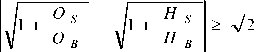
only when

O

1 + — S

O _B

H

1 + — S- H B

> 72.

In this occasion, the supplier’s inventory-related cost will be reduced.

Conclusion 1: In the case of supplier-driven supply chain, VMI can reduce the system’s(buyer and supplier together) and the buyer’s inventory related costs in the short-term, but the supplier's inventory related costs can be reduced if and only if

d_v ^* exists when the second-order condition is satisfied, then the optimal purchase price w_v ^* and the optimal selling price p_v ^* can be calculated out based on d_v ^* .

V. Effect of VMI on the profits of the supply

CHAIN

We can evaluate this effect by comparing the profits level before and after VMI under the optimal order quantity.

Effect of VMI on the system profits of the supply chain

• IV.    Effect of VMI on inventory related costs

The short-term effect of VMI is often the important reason for the parties to decide whether to continue applying VMI. In the early stages of VMI application, due to market constraints, agreements with other parties or balanced relationship, the sales and purchases are stable, that is, to maintain the level before the application of VMI, and the same to the selling price. In the short term, the effect of VMI is mainly reflected in the inventory-related costs.

Effect of VMI on the system inventory-related costs

The system inventory-related costs before application of VMI are:

I = I + 1 = J 2 h • О • d +| 0_s d-H B + H d ^ O ^I (14) B S     BB     S         S

2 O      2 H

BB

From (9) and (11), we know that:

R B ⁺ R S = P ^{( d}v ) • ^dv ^{- Cd}v ) V ^{2 ( 0}S ⁺ O B M ^HS ^{+ H}B ) • ^dv

From the first-order condition of (RVB + RS) at the point of dv = dv, we can obtain:

^d R/ R¹ . = p ( d * ) + p >( d v ) d v - c( d v ) -l ⁽⁰S ^{+ O b} ) •* H S ⁺ H B ) c (d v )    dv - d *                                Ц         2 d *

Subtracting the right of (13) from the left of (19), and the result is not less than zero when the first-order condition and second-order condition of the price function are not positive. That is, 2

^- P "⁽ d v ) d v ^{- 2} P X d v ) ^dv >  ^{0                 (20)}

And the system inventory-related costs after application of VMI are:

I v = I B + I S = 7 2 ( O s + O b ) • ( H s + H b ) • d v  (15)

Since

And d_v ^* is in the increasing interval of the function ( R B + R S ).

From (5) and (6),

I - I v

Id • h„ • О „ Г Г   ОТ   Г, Hs '

J---^B—B •   1 +- S - 1 +- S

V 2 А О \ H v 2 к V Ob 4 HB у

> 0

R = R B + R S = p ( d ) d - C ( d ) -V 2O B • Hb• d - O S dH B + H_s.

d • O B

к

O S   H S

So long as —— ^ ——, the system inventory-related O_B  H_B

Since

1 2H b J

costs can be reduced by VMI system.

R v ( d •) - R ( d •) = d d ^- H 2 B - O^B

•

O

1 + — O B

’ 1 + HS. I >  0 H b J

Effect of VMI on the supplier’s inventory-related costs

Although the buyer can achieve zero-inventory through VMI, the supplier's inventory related cost is possible to rise.

Since

R _v ( d * ) >  R ( d *)       when

d_v >  d

(22) (i.e.,

O

1 + —

O B

H S

1 +----> 1 ). But this is not critical condition.

_HB             notcrtcaco

, v ^d • ^Hb • O B s s \\ n

In addition, when the second-order condition of the price function is greater than zero, the discussion needs to do another.

I s - I S >  0

Effect of VMI on the profits of the buyer

From the first-order condition of R_B ^v at the point of d v = d v , we can obtain,

p "( d ) • d ² + 3 p '( d ) • d + p ( d ) - C ^,( d ) -J ^{( Os +} O ^B ) ^ ⁽ H S + H B ) 2 d

—

5 R B

5 d v

1 <  о H

■ p "( d ) • d + ³ p '( d ) • d + ^pd ^{) -} C ( d ) ^--l 1+7Г+77" U" _                               ² k ^OB H B/•

o_b • H_B

BB

2 d

. = P ( ^d V ) + P ' ⁽ d v ) d v ^- w v     (23)

dv = d*

Subtracting the right of (13) from the left of the (23), and the result is not less than zero when the first-order condition and second-order condition of the price function are not positive. That is,

*\л*2       *1/ I I ( O ⁺ O B ^)-( H - ⁺ H B )^0

^- p ⁽ d v )d v ^{- 2} p ⁽ d v )d v ⁺ C ⁽ d v ) ⁺ J-------- > 0

2 d_v ^*

And d _v is in the increasing interval of R_B ^v .

Since

R B ( d *) - R _B ( d *) = 7 2 O _B ■ HB ■ d* >  0         (25)

When

/

O S

= ¹ 1 ++

H

OH

BB

• 1    O_B • H_g

BB

• 2   2 d

/

•

к

O

1 +—

O B

VH J н

H B J

- 1

Therefore, when

O

1 +—

O B

H

1 +—-

H B

> 1 , type (28) is

not less than zero. And if (8) is satisfied,

p '( d ) - d *² + 3 p ( d ") - d + p ( d )-C( d *) -

( O S + O B ) • ( H - + H b ) 2 d ^*

**

d _v >  d (i.e.,

O

1 + —

O B

> 1),

> p '( d ) - d *² + 3 p ( d ) - d + p ( d *) -c ( d ) - 2

1 +

к

O + H 1 OiH

OH

BB

= 0

R B ( d_v ) - R b ( d ) > R B ( d ) - R b ( d ) = V 2O b • H b - d > 0

That is, R B ( d_v ) >  R_B ( d ) . But this is not critical condition. In addition, when the second-order condition of the price function is greater than zero, the discussion needs to do another.

Since the first-order condition of the profit function is

OS a decreasing function, in case of 1+ OB

1 + H^- > 1 ,

H B   ,

d_v >  d , and on the contrary , d_v <  d .

Effect of VMI on the profits of the supplier.

*

d_v is the maximum point of the supplier’s profits

Conclusion 3:

When

after application of VMI, thus,

R s (d * ) - R s (d) >  R s ( d ) - R s ( d ) =

F O C H i

1 +- S - 1 +- S I

J O B 1 H b J

- 2

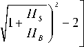
And R - ( d * ) >  R_s ( d * ) when

Conclusion 2: In the case of supplier-driven supply chain, VMI can increase the system’s and the buyer’s

**

profits when d _v >  d (i.e.,

when

O

1+о

H

1 + —-

H B

O

1 + —

O B

H

1 + -f- >  1 ).And H_B

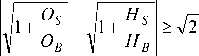
> V2 (Non-stringent threshold

condition) , the supplier's profits can be increased.

VI. Effect of VMI on the total annual PURCHASe amount of the supply chain

From (8) and (13), we know that:

O

1 + - S

O B

H

1 + — S

H B

> 1 , the

implementation of VMI can increase the total annual purchase amount of the supply chain.

VII. EFFECT OF VMI ON THE PURCHASE PRICE OF THE SUPPLY CHAIN

From (7) and (12), we know that the difference between the purchase price before and after application of VMI is:

W v - w = p ' ( d v ) - d v + p ( d v ) - p ' ( d ) - d - p ( d ) +. H B O B

2 d (30)

When d_v = d , w_v - w = ₄ H B ' O B >  0 . v v            2 d

Conclusion 3: In the short term ( d_v = d ), VMI can increase the purchase price. But in the long term ( d_v ^ d ), it depends on the relationships between d_v and d , as well as the features of function p ( d ) .

• VIII. Calculation case

Calculation case

We assume the price function is p ( d ) = a — b • d , ( a , b >  0) , and the supplier's cost function is C ( d ) = 5 • d + 0.50 • d 2 , (5,0 >  0) . Please note that C '( d ), C "( d ) >  0, p '( d ) <  0 . This case is cited from [4] based on the relationship of VMI between a telecom equipment manufacturer (as supplier) and its customer. In this case, the manufacturer's order cost is O S = 1500 (USD) and inventory holding cost is H S = 9 (USD / year • unit). The buyer's ordering cost is O B = 300 (USD) and inventory holding cost is H B = 9 (USD / year • unit). [4] (The parameters values see Table I ).

TABLE I.      P arameters sheet of the specific case

Parameters	a	b	5	0	Os	O B	H S	H B
Value	80	0.01	40	0.005	1500	300	9	9

We can obtain the results using the established model and the corresponding MATLAB program (see Table II).

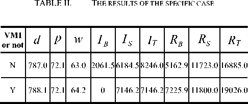
From the data of Table II , we know that in the supplier-driven supply chain, the total system profits are increased and the total inventory-related costs are decreased significantly under VMI.

Simulation

The VMI’s effects on supply chain performance contact closely to the cost structure between the two

HS     OS parties (i.e., the relationship between and ). HB     OB

Furthermore, the cost structure is one of the factors most likely to change in supply chain. In order to test the foregoing conclusions and search for the trend of VMI effects on supply chain performance with the variation of supply chain cost structure, we will do some simulation analysis for the costs, profits and other indicators. The following variations of OS will be representative of the cost structure changes (the increase of OS on behalf of the increase of stock structural differences between the two parties). (Results shown in Table Ш).

TABLE III.     C alculation sheet of supplier - driven supply

CHAIN

O S	VMI Or not	d	p	w	I B	I S	I T	R B	R S	R T
0	N	861.1	71.4	61.5	2156.4	1078.2	3234.6	6336.7	17272.0	23609. 0
	Y	849.3	71.5	63.0	0	3028.6	3028.6	8477.0	16337.0	24814. 0
300	N	846.8	71.5	61.8	2138.4	2138.4	4276.8	6101.5	16144.0	22245. 0
	Y	832.3	71.7	63.4	0	4240.0	4240.0	8219.5	15024.0	23244. 0
900	N	817.5	71.8	62.4	2101.1	4202.1	6303.2	5632.5	13914.0	19547. 0
	Y	807.6	71.9	63.8	0	5906.6	5906.6	7719.9	13190.0	20910. 0
1500	N	787.0	72.1	63.0	2061.5	6184.5	8246.0	5162.9	11723.0	16885. 0
	Y	788.1	72.1	64.2	0	7146.2	7146.2	7225.9	11800.0	19026. 0
2100	N	755.2	72.4	63.6	2019.4	8077.7	10097.0	4693.6	9571.5	14265. 0
	Y	771.3	72.3	64.6	0	8163.4	8163.4	6731.9	10642.0	17374. 0
2700	N	721.7	72.8	64.2	1974.1	9870.6	11845.0	4221.4	7463.1	11685. 0
	Y	756.1	72.4	64.9	0	9036.5	9036.5	6230.8	9630.8	15862. 0

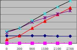
• 1)    The variation of inventory-related costs under different cost structure.

12000 10000 8000

I 6000 4000 2000 0

Os

IB before

IB after

Is before

Itotal after/Is after Itotal before

Figure 1. The variation of inventory-related costs under different cost structure

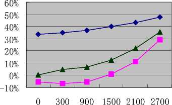
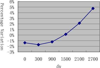
Figure 2. The percentage variation of inventory-related costs under different cost structure

Fig. 1 and Fig. 2 show that with increasing of ^S , the system inventory-related costs and the supplier’s have gradually increased, the buyer’s inventory-related costs decreased slightly before VMI and reduced to zero after VMI. Under different cost structures, the buyer’s and the system’s inventory-related costs are reduced before and after the application of VMI, but the supplier's inventory-related costs may be increased or reduced. From the percentage variation, we can see that with increasing of the cost structure difference, the supplier’s inventory-related costs increase slowed down and the variation percentage changes from positive to negative. The variation percentage of the system inventory-related costs is always in negative territory, and its trend line is an increased to decreased curve. And the variation percentage of the buyer's inventory costs is always 100%.

• 2)    The variation of profits under different cost structure.

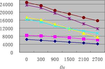
- ♦ RB before     —■ Rb after

Rs before           Rs after

■ж Rtotal before —• Rtotal after

Os

— ♦ — Buyer —■ Supplier —*— System

Figure 4. The percentage variation of profits under different cost structure

Fig. 3 and Fig. 4 show that, with increasing of ^S , the profits of both parties trend to be reduced. Under different cost structure, the system’s and the buyer's profits are always increased after the application of VMI, but the supplier’s profits may be increased or reduced. From the variation percentage of the profits, we can see that with increasing of the cost structure difference, the increased percentage of the buyer’s and the system’s profits gradually increase. The variation percentage of the supplier's profits change gradually from negative to positive after the application of VMI, and its trend line is a first slightly reduced and then increased curve.

• 3)    The variation of perchase amount under different cost structure.

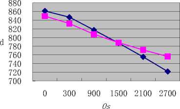
before after

• Figure5.    The variation of purchase amount under different cost structure

Figure 3. The variation of profits under different cost structure

Percentage of difference

• Figure6.    The percentage variation of purchase amount under different cost structure

Fig. 5 and Fig. 4 show that, with increasing of ^S , both of the purchase amounts before and after VMI trend to be reduced. That is due to increasing of contract purchase price w along with costs rising, which caused a chain reaction between buyer and supplier, as a result of the eventually the annual demand reduction. Under different cost structure, the purchase amount may be increased or reduced after the application of VMI. From the variation percentage of the purchase amount, we can see that with increasing of the cost structure difference, the changes of purchase amount turn from negative to positive, and the percentage variation shows a slightly decreasing trend when O_S is very small, then it trends evidently to increase.