About non-parametric identification of partial-parametred discrete-continuous process

Introduction. In numerous occasions for many technological, manufacturing, and multidimensional processes of a discrete-continuous nature, researchers are put in conditions where it is necessary to build a model of the process under study. These processes are dynamic in nature, but controlled at discrete intervals, including different ones, which results in dynamic processes to be seen as inertia-free with a time delay. For example, when grinding any materials (clinker, coal), the time constant is 5–10 minutes, and the control of the output variable, such as the fineness of grinding, is measured every two hours. In this case, the investigated process can be presented as inertia-free with delay [1].

Similar processes are often found in mining or processing industries, such as metallurgy (steel smelting), power industry (coal burning), construction (cement production), oil refining (diesel purification) [2], and social sciences, including education (student learning) [3].

However, the most interesting and important thing is that while researching different processes there is a class of processes that is classified as T-processes [1]. Similar processes have stochastic dependence of output variables and require alternative methods of identification and control, slightly different from conventional ones. The main thing here is that identification of such objects should be carried out applying non-traditional for the existing theory of identification methods [4]. It is also interesting for the cases where a priori information corresponds to both nonparametric and parametric types of raw data on the process under investigation. Such processes are classified as KT processes [1].

A special feature of KT-processes is that equations of relations between input and output variables with accuracy to the vector of parameters are known for some channels of the multidimensional system, but are not known for the other channels, causing the fact that the mathematical description of the object is presented in the form of some analogue of the system with partially parameterized F j ( u , x , a ) = 0, j = 1, n and unknown functions with the view F j ( u , x ) = 0, j = 1, n . Thus, the problem of identification is reduced to the problem of solving the system of nonlinear equations of a partially-parameterized discrete-continuous process with respect to vector components, and known values of input variables u. Specific identification tasks will diverge by different amount of a priori information on different channels, and by the features of ongoing processes. What is important here is that we have to face a system of different equations in terms of mathematics, the solution of which will require development of special methods. In this case, it is advisable to use methods of non-parametric statistics [5; 6].

KT-processes. Currently, the role of inertia-free systems with delay identification is increasing [7; 8]. This is because some of the most important dynamic object output variables are measured at long intervals of time, far exceeding the time constant of the object.

Let’s consider a general scheme of a discrete-continuous process that functions under conditions of diverse a priori information, including non-parametric uncertainty, which is consistent with identification theory in a broad sense.

A feature of multidimensional object identification is that the process being investigated is described by a system with implicit stochastic equations.

F j ( u ( t -t ) , x ( t ) , ^ ( t ) ) = 0, j = 1, n ,       (1)

Where on some channels F j ( ■ ) are unknown, and on other channels are known, t - on different channels of multidimensional system [1]. Further, for simplicity t will be omitted.

In general view, the investigated multidimensional system implementing the KT process can be shown in fig. 1.

In fig. 1 the following symbols are set: u = ( u 1 ,..., u m ) - m -dimensional vector of input variables, x = ( x 1 ,..., x n ) - n -dimensional vector of output variables, £ ( t ) - random interference influencing the process, vertical arrows indicate stochastic dependence of output variables, arc arrows show internal connection between variables, which is characteristic of a specific investigated process. Clearly, the nature of some relations remains unknown to the researcher.

Through various channels of the process under study, the dependence of the j component of vector x may be represented as some dependence on certain components of vector u : x < ^j >  = f j ( u < ^j > ) , j = 1, n . Such functions are determined by the researcher on the basis of available a priori information and are called a composite vector. A composite vector is a vector composed of some components of the corresponding vector, u < ^j > = ( x 2 , x 5 , x 7 , x ₈ ) in particular. It may also be any other set, for example, u <5> = ( u 1 ,u 3 , u 6 ) where u < 5 > is a composite vector, or x <³> = ( u 1 , u 3 , x 2 ) . In this case, the system of equations becomes:

' F ( u <> , x < ^j > , a ) = 0,

F 2 ⁽ u < ^j > , x < ^j > , ^a ) = 0, _

« ... j = 1, n , (2) F n —1 ⁽ u < ^j > , x < ^j > ) = 0,

_ F n ( u < ^j > , x < ^j > ) = 0.

where F j ( ■ ) partially parameterized or unknown, a is a vector of parameters.

KT-models. Multidimensional processes which output variables acquire unknown stochastic relationships were called T-processes, so their models are respectively called T-models [1]. K-models are based on the use of diverse a priori information across different channels of a multidimensional object.

A KT model combines T-model elements with K-model elements and is a model in which there is a set of relationships between input and output variables, where dependences are known through some channels, for example, by focusing on the laws of physics, but unknown in other channels.

The main feature of modeling such a process in conditions of non-parametric uncertainty is the fact that the type of functions F j ( u < ^j > , x < ^j > ) = 0, j = 1, n is known for one certain channel and unknown for another. Naturally, the model system can be presented as follows:

F 1 ( u <  j > , x <  j > , a ) = 0;

F ( u < j > , x < j > , ^a ) = 0;        _

«...                                    j = 1, n , (3)

^F n -1 ( ^u <  j > , ^x <  j > , x s , j? s ) = 0;

F ^ n ( u < j > , x < j > , x s , u s ) = 0.

where x _s , й _s - time vectors (a data set, obtained by s-time point), in particular          x _s = ( x 1 ,..., x _s ) =

^{( x} 11 , ^x 12 ,..., ^x 1 s

x ₂₁, x ₂₂

x2s ,...,xn1,xn2,..., xns ) , but in this case some F^j (■), j = 1, n remain unknown. There- fore, let’s consider the task of constructing KT models under non-parametric uncertainty that is under conditions where the system (3) is known for some channels and is not accurately known for others.

So let the input of the object receive input variable values, which are certainly measured. The presence of a learning sample x i , u i , i = 1, s is necessary. In this case, estimation of the components of the output variable vector at known values, as already mentioned above, causes the need to solve the system of equations (3).

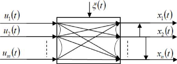
Fig. 1. Multidimensional system

Рис. 1. Многомерная система

In case the dependence of the output component on the component of the vector of input variables is not known, it is natural to use non-parametric estimation methods [9; 10].

The problem is that with a given value of the input variable vector u = u ' , it is necessary to solve the system (3) with respect to the output variable vector x . For some channels of the multidimensional system, where equations accuracy within parameters is known, coefficients are found, for example, by the method of stochastic approximations [11]. For other channels where relations are unknown, the following algorithm chain [1] must be applied. First, inconsistencies are calculated by formula:

^£ У = ^F j ( ^U <  j >  , x <  j > ( i ) , x s ," s ) , ^j = 1, n , ⁽⁴⁾

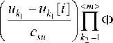
where F ( u < ^j > , x < ^j > ( i ) , X _s , u _s ) is accepted as nonparametric estimates of Nadarai-Watson regression [12]:

j i ) = F j ( ^u < ^j > , x j ⁽ i ) ) =

= xj( i)-

s        <  n >

Z X j [ i ] П Ф i =1          k =1

' u k - u k [ i ] '

c

к       suk      7

s <  n >

Zn Ф

i =1 k =1

' u k - u k [ i ] '

к     suk    7

where j = 1, n , , <  m >  - composite vector dimensions

u _k

. Bell curve function Ф

' u k - u k [ i ] ' к     ^su k    7

and blur parame-

ter c _suk comply with some convergence condition, so obtain the following:

Ф ( ■ ) <-» ; ^c ' j Ф ( ^c / ( ^u - ^u_i')^d^u = 1;      (6)

Q ( u )

^lim s ^» ^c ' Ф ( ^c k ( ^{u -} u ) ) = 8 ( ^u - ^u i ) , ^lim s ^» ^c s = 0, ^lim s^ ^sc s = ” -

Next step is estimation of conditional mathematical expectation:

X j = M { x | u < ^j > , s = 0 } , j = 1, n .         (8)

As estimate (8) we accept non-parametric estimate of Nadarai-Watson regression [12]:

x j =

s         <  n >

Z X j [ i ] ■ П Ф i = 1            k ₁ = 1

[^

к ^cs =

s < n > zn Ф i=1 ki=1

< m >

П ^Ф k 2 = 1

j = 1, n ,

к

/

where bell curve Ф ( ■ ) may be accepted in the form of triangular kernel (10) and (11), complying with the conditions (6), (7).

₁   |^uk ^{- u} k ^[ i ^]|   | ^u k ^{- u} k ^[ i ^]|   ₁

1 —^L, ^L< 1 ^c su              ^c su

| ^uk 1 - ^u k 1 ^[ i ^]|

,.

1 -

0,

10 -= k ₂ [ i ] 10 -= k ₂ [ i ]|

10 -=-.и| > 1

< 1,

Algorithms (5), (8) and (9) are an algorithm chain necessary to calculate the prediction of the components of the output vector under the known input components [1].

While carrying out this procedure, we obtain values of output variables x at input influences on the object u = u ' , which is the main purpose of the desired model that can further be used in different control systems [9], including organizational systems [3].

The accuracy of the simulation is estimated by the following formula:

s

Z|xi - xs (ui )|

8 = ^=---------- s

Zlxi- X i=1

where x i - object observation, x _s ( u i ) - object output forecast, x ˆ – average value for every vector component x .

Computational experiment. An object with five input variables u = ( u ₁, u ₂, u 3 , u ₄, u 5 ) , and three output variables x = ( x ₁, x ₂, x 3 ) , was taken for the computational experiment. For this object, a sample of input and output variables was formed based on the system of equations of two parametric and one non-parametric channel. As a result, a learning sample was obtained u _s , x _s , where u _s , x _s are time vectors. If the task was to be solved for a real object, the learning sample would be formed as a result of measurements carried out by the available control means. In the case of stochastic dependence between output variables, it is natural to describe the process, for example, by the following system of equations:

F⁷ x 1 ( ^x 1 , ^x 3 , ^u 1 , ^u 2 , ^u 5 ) = 0;

*F x 2 ( ^x 1 , x 2,^u 4 , ^u 5 ) = 0; ⁽¹³⁾ _ F⁷ x 3 ( ^x 1 , x 2 , x 3 , ^u 2 ,^u 3 , ^u 5 ) = 0.

Once a sample of observations has been obtained, it is possible to proceed with the task under study – to find the forecast of the values of the output variables x under the known input u. For the case where there was an equation dependency across the two channels, the coefficients were found applying the stochastic approximation method.

To begin with, the inconsistencies are calculated according to the procedure described above. Let us present the inconsistencies in the form of a system:

8 1 ( i ) = F ( x i , x 3 , u l , и , u 5 ) ;

" ⁸ 2 ^{( 1} ) = F 2 ( x l, x 2 , u 4 , u 5 ) ;

⁸ 3 ( ¹ ) = F 3 ( x l , x 2 , x 3 , u 2 , u 3 , u 5 ) .

where 8 j , j = 1.3 - inconsistencies, for which corresponding components of the output vector cannot be obtained from parametrical equations.

Forecast for system (13) is performed according to formula (9) for each component of object output.

Input variables of newly generated input variables, i. e. not included in learning sample, are supplied to object input.

The tunable parameter will be the blur parameter, which in this case will be taken to be 0.4 (the value was determined as a result of numerous experiments to reduce the quadratic error between the output of the model and the object) [13; 14], the blur parameter will be taken the same when counted in formulas (5) and (9), sample size 5 = 2000, interference ^ = 0.07 . By component, we provide graphs for the object outputs x1,x2 and x3 .

In fig. 2–4 ‘X’ shows the values of the variable output and the point of the model output. The figures demonstrate a comparison of the test sample output vector components true values and their predicted values obtained using algorithm (5)–(9). The figures show 20 sampling points due to the simplicity of results presentation, i. e. each one-hundred sampling point. The figures show that the model describes the object quite well at the interference of 7 % acting on the components of the output variables.

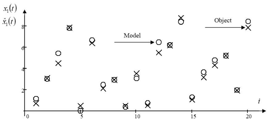
Fig. 2. Forecast values of the output variable x ₁ with interference 7 %

Рис. 2. Прогнозные значения выходной переменной x ₁ при помехе 7 %

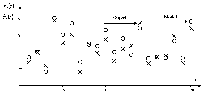
Fig. 3. Forecast values of the output variable x ₂ with interference 7 %

Рис. 3. Прогнозные значения выходной переменной x ₂ при помехе 7 %

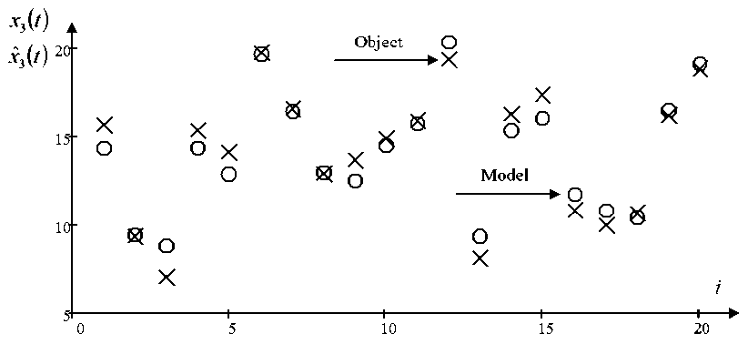
Fig. 4. Forecast values of the output variable x ₃ with interference 7 %

Рис. 4. Прогнозные значения выходной переменной x ₃ при помехе 7 %

In fig. 3, the prediction of the output variable is slightly worse than for the rest of the output variables, this may be affected by: the quality of the learning sample, the dependency of the variables, random interference, blur parameters, etc.

Conclusion. In the present work, the problem of identifying partially parameterized retarded multidimensional objects has been discussed. A number of features which appear include the fact that the identification task is considered in conditions of non-parametric uncertainty and, as a consequence, cannot be presented with precision to a set of parameters. Such processes can be well used in various control systems [15]. Based on the available a priori hypotheses, the system of equations describing the process is produced using composite vectors x and u. However, functions F ( ■ ) continue to be unknown for some channels. The article discusses the method of calculating output variables of an object with known input variables, which allows to use them in computer systems of various purposes.

It should also be noted that KT models have found their application in the actual catalytic hydrodepaffiniza-tion process (or diesel purification process) and, as a result of computational experiments, have produced sufficiently satisfactory results [2].

Numerous computational experiments have shown quite satisfactory KT simulation results. Issues related to the introduction of different interferences, different volumes of learning samples were studied, as well as objects of different dimensions were investigated [4].