About the analysis of the pulse-width system with feedback

Pulse-width systems (PWS) find application in automatic control devices, as well as in amplifiers of capacity of “D” class with an intermediate pulse-width modulation, captured by a negative feedback for the reduction of nonlinear distortions. Feedback presence in PWSs is inevitably connected with the problem of stability maintenance. The solution of this problem, in a comprehensible with practical application way for the PWSs generally does not exist. The possibilities of private decisions have been considered in [1; 2].

The aim of the present work consists in the search for new methods of the PWS stability analysis, applicable in practical applications.

Methods of pulse-width systems analysis. An analysis of the pulse systems is made, as a rule, basing on the theory of trellised functions and discrete transformation of Laplasa [1]. The theory of pulse-amplitude systems has now developed in enough detail: for a linear path and for systems containing nonlinear inertialess elements [1; 2].

Unlike the АPS, the PWS is much more difficult to analyze, therefore it is investigated using data equivalent to the nonlinear АPS.

A nonlinear АРS block diagram is presented in fig. 1.

Fig. 1. The block diagram of a nonlinear АPS:

f ( t ), z ( t ) – are the input/output signals; w ( t ) – is the pulse characteristic of the PWS continuous (linear) part; γ – is the duration of an impulse; x ( t ) – is the error signal; y ( t ) – is the nonlinear transformation x ( t ); 1 – nonlinear inertialess tract converters; 2 – the generator clock δ – are the functions modulated on amplitude by signal y ( t ); 3 – the generator of form impulses s ( t );

4 – a linear part of a path

According to [2], the formula of the control systems (fig. 1) looks as:

x(n,0)=f(n,0)-BT× n=1         γ

∑ Ф( x ) ∫ S ( τ ) ω ( n - m - 1,1

- τ ) d τ ,

m = 0

τ where τ =   – is the discrete time; B – is the coefficient

T of linear strengthening x(t) in the APS tract.

The integral in (1) represents the convolution of the function for a forming element and the pulse characteristic ω( t ). In the research [2] this has received the name of the resulted pulse characteristic ω( t ).

If equation PWS manages to be reduced to (1) to it is possible to apply all known methods of the analysis and calculation of nonlinear АРS.

A simplified block PWS diagram is presented in fig. 2.

For PWS the function of a forming element s ( t ) looks like fig. 3, where Т – is the period of clock frequency.

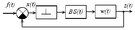
Fig. 1.2. The block diagram of the PWS

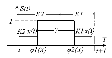
Fig. 1.3. Forming the PWS element

According to fig. 3, s ( τ ) corresponds to the bilateral PWS.

In К 1 = 0, or К 2 = 0 the unilateral takes the place of PWS.

By analogy with (1), for PWS it is possible to write down following expression:

x ( n ,0) = f ( n ,0) - BT ×

n-1 ϕ2 (χ)                                                     (2)

× ∑ ∫ S ( τ ) ω ( n - m - 1,1 -τ ) d τ .

m = 0 ϕ 1( χ )

Unlike (1), the integral in (2) is functioning and x ( t ), defines the features of the PWS analysis.

Accorging to fig. 3

Ф 1 ( х ) = К 2 (1 - х ); ф ₂( х ) = К 2 + К 1 х ;

К 1 + К 2 = 1.                     (3)

Let’s include the concept of factor of PWS symmetry,

А = К К , К 1 + К 2

К 1 = 1 + А ; К 2 = ЦА .         (4)

On an integration interval in (2) 5 ( т ) = 1, and ω ( n – m– 1; 1) it is possible to present a number of elementary pulse characteristics:

Comparing (7) and (1) it is possible to draw a conclusion that the PWS it is reduced to the equivalent multidimensional nonlinear APS.

The number of parallel branches equivalent to the APS is equal to the number of roots in the typical equation.

The analysis of the multidimensional nonlinear APS allows us to define only the absolute stability of the system in a general view; the results comprehensible to practical management are to be received only for twodimensional systems, or for systems reduced to twodimensional during the stability analysis [3].

In this case the analysis of PWS stability resorts to the approached methods, allowing the decrease in the APS order equivalent. In [4], for example, it is offered to present Ф ν ( x ) as a sedate polynom of such a kind:

5 rv - 1

V Ц v = 0 Ц= ⁰

ш ( n - m - 1,1 - т ) =

( n - m -т ) ^ц

-----ц!-----exp

q v ⁽ n - m ^-t )

N

Ф v ⁽ % ) = Z r k(^v ) % ^k . k = 1

In this case (7) becomes:

where s – is a number of different poles; r ν – is the frequency rate v of the poles:

C' =        1          d ( rv ^{-ц- 1)}

^{v ц} = ( r v -ц- 1)! ' dq ⁽ r^{v -ц- 1)}

Р Н ( q ); Q H ( q ) – are the polynoms in the numerator and a denominator of the transfer function of continuous part of the PWS W ( q ) .

Let’s assume that all poles are simple and are not equal to zero (the presence of zero or multiple poles does not complicate and does not simplify a problem of the PWS and APS data.

For a case with simple poles:

P_H ( q )          _r

---------( q - q ) ^v

TQ H ( q )      ^v

n - 1 5 N

% ( n ,0) = f ( n ,0) - BT ZZZ C v e xp L q v ( n - m ) Jx m = 0 ^v = 1 k = 1

n - 1 N

X %k (m,0)=f (n,0)-BTZ Z %k (m,0)®Пk (n-m), m=0 k=1

,

< = Cv = IW (q)(q - qv )L q qv

s '

m( n - m -1,1 - т) = Z Cv exp v=1

q v ⁽ n ^- m ^-t )

Substituting (6) in (2), we will receive:

n - 1 ⁵

% (n ,0) = f (n ,0) - BT ZZ m=0 v=1

where:

Ф 2( х )           _ _

J exp - q т d т ф^ х )      L J

'

X C v exp [ q v ( n - m ) ] = f ( n ,0) - BT x         (7)

n-1 I t ._                 -I                           I x Z{Z Ф v L %(m ,0)J wПv (n -m)(..., m= 0 v=1

Ф 2[ % ( m ,0)]

Ф v [ % ( m ,0) ] =    J exp

Ф 1[ % ( m ,0)]

- q_v т d т

W П v = C v exp [ q v ( n - m ) ] .

where:

N

^' nv ⁽ n ^- m ) = Z r ( ^v ) C v exp [ q v ^{( n - m} ) ] - ⁽¹²⁾ v = 1

When comparing (7) and (11), it is easy to notice that in (11) the number of branches is linear and is defined by the number of polynom members (10), from which it occurs.

If the equivalent nonlinearity Ф ν ( x ) is rather small in a polynom (10) it is possible to leave only two or three composed. Thus, the equivalent APS will be two – three measurements, even in case of constant usages of linear PWS parts.

If: Ф _v ( % ) = r 1 ^{( v} ) ■ % + r ₂ ^{( v} ) ■ % ².

As shown in [4], the PWS block diagram can be shown as a one-dimensional nonlinear APS.

Such a method of approached analysis of stability is especially effective, when the nonlinearity equivalent APS is expressed poorly.

The analysis of PWS stability; the method of artificial order drop in its linear part. The approached calculation of transients is based on an offered method of the analysis in difficult linear chains. This way is offered and in details investigated by J. S. Itshoki [5]. Its issues are following:

The order of the initial differential equation of a linear part of the system artificially goes down (the differential equation “is shortened”), and equivalent delay (in certain cases probably and not a late decision) is placed into the system description.

The parameters of the truncated equation steal up so (fig. 4), that a steepness of transitive function increase h ( t ) in in-between decline space (DS) and the amplitude of the

oscillatory process (if possible) corresponds to the initial h ( t ).

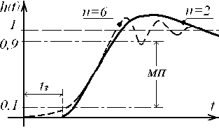
Fig. 4. Approximation of the transitive feature

In case when m = 2, two variants are possible:

• 1.    Approach m = 1 does not exist, i. e. Δ2 ≥ 0,5Δ12. The condition of the existing approach m = 2 looks like: A  A,   1

• 2.    Approach m = 1 exists, but the accuracy of approach is insufficient. Then the condition of approach existence m = 2 becomes:

— < —---.

A 3    a 2 з

A- < a3

i+

3 3 к    A 2 J

11 Ai ]

2 (a? J

1    a2    1 ( a2 ]

1 + -2- +    2

3A1  4 U? J

Such a method can be rather effective even during the fall of difficult linear chains of a high order to the first and the second order.

For the solution of the approached description of the PWS linear part, its transfer function is necessary to lead the normalized equation to:

W ( p ) = ^{1 +} g . p ⁺ g 2 p ' ⁺ L ^{+ g}n p " .

1 + a1 p + a 2 p2 +— + akp

Where at least n < k – 1 (at n > k – 1 the approximation by late function does not exist).

The required approximation W ( p ) in order m is found in:

Because the increase of an approximation order sharply complicates a problem of search for the approached decision and the analysis of PWS stability, it is not necessary to apparently use, m > 2.

Let’s assume that in result of the considered method of approximation PWS linear function in the form of the first order approach ( m = 1) is defined:

W ( p ) =

exP [ ^- pt 3 1 ]     1 exP [ ^- pt 3 1 ]

--------=------ ^{1 + b} 1 ‘ p     ^b1     p ₊1

^p b

Wm ( p ) =

exP [ - pt 3T ]

1 + bp + b 2 p ² + L + b m p m

where t_зт – it is defined by the solution of the following equation:

The corresponding trellised (discrete) pulse characteristic on the basis of (6) will become:

w (n - m - k, k - т - -1) =

= b 1 ex^P

1 (

- —( n - m - k ) exp

-

—(k-T b1

-

where:

, m + 1

t зт

( m + 1 ) !

t ^m

- 3^- + L +

m !

(-1) m +1

'^A m + 1

= 0,

^A 1 = ^a 1 ^- g 1 , A ₂ = a 2 ^{- g} 2 ^- a 1 ■ ^g1 ,

where - 1 = tT ; b 1 = T^; k - comes out such, that it makes time discrete time.

The resulted pulse characteristic according to (9) can be written down as:

^A 3 = a 3 - ^g 3 - a 2 ■ ^g 2 - a 2 ■ ^g 1 .

Let’s notice that necessary value of delay tз corresponds to the least material (always positive) root t з = t зm . Finding this value it is uneasy even at m = 3.

Other parameters of approximation in (13) are found as follows:

w n 1 = Г ^exP b ₁

- b- (n - m -1)

■ exP

-

Г ( 1 - - 1 ) . ^b 1           _

Nonlinearity equivalent APS we will be according to (8):

b1 = A1 - -зт зт b2   A2  A1 t зт + 2!

K 2 + K 1 X

Ф1 [ X (m ,0 )_=  J exP к 2 (1-X)

1 "

— т d т = b ₁ _

= ^b 1

exP b ¹ ( ^K 2 ^{+ K} 1 ^X )

- exP K- (1 - X)

b' =Am -Am^1 + Am-2 ■ t3T-......+ (-1)mt-^- m 1!         2!                      m!

For the approximation of this or that order there are certain living conditions.

Order approach m = 0 exists always.

Approach m = 1 is limited by a condition A. <  2.

where X – has normalized a signal changing within 0 <  X < 1. Taking into account, expression can be copied as so:

Ф 1 ( X ) = 2 b 1 exP

-b, <‘ - A >

■ exP

AX XX sh

2 b 1 J 2 b 1

Schedules of this dependence for each special case b ₁ = 0.5 are presented in fig. 5. As one would expect, at

asymmetrical kinds PWS ( А = ±1) nonlinearity Ф₁( x ) -expresses not much more strongly, than in А = 0.

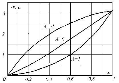
Fig. 5. Nonlinear PWS characteristics

— + Re

CT

^{exp -} | Г ^- t 1 )

B L b J ■ bi        r • Г 1

exp [ jw ] - exp

> 0,.

where

д Ф₁ ( x )

is the maximum differential

value of factor of equivalent nonlinear element transfer.

In – is the factor of linear strengthening in the PWS pulse tract.

Introducing the connecting processes, offered by L. S. Iuhoni, the method drawn near calculation, has greatly allowed simplifying the problem of the analysis to a stable width-pulsed system in the event of a high order even by its linearities.

The transfer function of the resulted linear part will be found in the form of discrete Laplasa transformation from (14):

w:( q ,0 ) = b1

exp

b<" - -1)

exp [ q ] - exp

Having replaced in this expression q by j (= и Т), we shall receive the peak-phase characteristic of the resulted linear PWS part. Using this detail, it is possible to estimate the PWS stability applying the criteria For example, according to criterion of the absolute position stability balance [2]: