Accelerated algorithm for calculating spectra of aperiodic gratings

One of the primary approaches to solving the scattering problem for the Helmholtz wave equation is the transfer matrices method (TMM), also known as the T-matrices method [1]. TMM is extensively utilized in computer optics for calculating laser mirrors, optical filters, and antireflection elements [1, 2]. Recently, TMM has become increasingly important for calculating scattering spectra in fiber Bragg gratings (FBGs), which are critical in optical communication lines, fiber lasers, and modern fiber-optic measurement systems, sensors, and detectors [3–7]. The calculation of FBG spectra for cascade gratings [8], gratings with chirp, and apodization [7, 10], which exhibit fine spectral structures, often requires substantial computational time. This necessitates the development of efficient numerical algorithms that are both fast and accurate, particularly for aperiodic gratings and gratings with deep modulation [9] where the coupled mode approximation fails, and solving the Helmholtz wave equation becomes imperative.

TMM reduces the direct scattering problem to the multiplication of transfer matrices. The accuracy and efficiency of the method depend on how the matrices are calculated and the speed at which their product is computed. The calculation of transfer matrices is based on the discrete approximation of the scattering problem. Basic methods that approximate the scatterer using discrete layers with constant refractive indices result in first-order accuracy algorithms, which demand relatively large discrete grid sizes and a substantial number of arithmetic operations to achieve high accuracy. The order of accuracy here refers to the degree of dependence of the calculation error (residual term) on the grid step size. Higher orders of approximation accuracy complicate the algorithm but reduce the required number of operations and the discretization size. Integral approaches to discretization, such as the finite volume method [11], provide high approximation accuracy and stable calculation schemes. However, the speed of the TMM algorithm for solving the spectral scattering problem can be further enhanced using modern numerical techniques such as the duplication strategy and the fast Fourier transform (FFT) [12]. These advanced approaches to the spectral scattering problem for the Helmholtz equation are the focus of this paper.

1.    Statement of the scattering problem

We begin with the one-dimensional Helmholtz wave equation for the electric field E ( x ) of a wave with wave vector k in a vacuum, for a scattering object with a coordinate-dependent refractive index n ( x ):

• ^dE + k ² n ² E =0.                            (1)

dx ²

Now, we represent the field E ( x ) as a sum of waves traveling left and right, in the case of volume Fresnel reflection [13], with oscillation amplitudes that satisfy the Bremmer transformations [14]:

E ( x ) = ^{Be i s + Ae - i s} , ^dE =i kn ( Be ^{i s} - Ae ^{- i s} ),   (2)

kn dx where i is the imaginary unit, s = kξ, and ξ is the optical coordinate, which for dielectric medium is one-to-one related to the geometric coordinate x by integral relations:

x                               ξ 1

• ξ ( x )= ∫ ₀ n ( x ′ ) dx ′ , x ( ξ )= ∫ ₀        d ξ′ .              (3)

n ( ξ )

For the oscillation amplitudes A and B , substituting relations (2) into the Helmholtz equation (1) gives the following pair of first-order differential equations:

dA = B ( ^ ) q ( ^ ) e -2i k ⁵ , dB = A © q © e 2i k ⁵ , d 5                   d 5

where the parameter q ( ^ ) =(1 / 2 n )( dn / d 5 ) is called the mode coupling coefficient (MCC). The MCC acts as the scattering potential in the scattering problem. The wave amplitudes of the waves traveling left and right, as functions of the optical coordinate ^ , are given by:

u © = Ae -i s = A ( ^ ) e -i k ⁵ , v © = Be i s = B © e i k ⁵ . (5)

Note that the amplitudes A and B also depend on the wave vector k as a parameter.

The boundary conditions for the scattering problem are based on the asymptotics of the solutions far from the scatterer. Specifically, we consider the right scattering problem, where the left-traveling wave u ( ^ ) is incident on the scattering object from the right, generating a right-traveling reflection wave v ©. The asymptotics of the wave amplitudes far from the scatterer are:

( u , v ) U^-„ = ( e i k ⁵ , 0), ( u , v ) , = = ( a ( k ) e -i^{k 5} , b ( k ) e i ^{k 5} ).

Here, a ( k ) and b ( k ) are the spectral scattering coefficients for the incident wave and the wave reflected from the scattering object,and the transmission coefficient is normalized to unity ( d ( k ) = 1). The coefficients a ( k ), b ( k ) determine the spectral reflection coefficient, which needs to be found:

r ( k ) = b ( k ) / a ( k ). (7)

The Fourier transform of the spectral reflectance provides the pulse response of the scatterer:

R ( x ) = — [ r ( k ) e -ikx dk . (8) 2 n^J-"

The following sections present an optimized numerical algorithm for solving the direct scattering problem, which involves determining the reflection coefficient r ( k ) across the entire significant spectral range of wave vectors k for a given refractive index x ( k ) of the transparent dielectric scatterer.

2. Discretization of the problem

We consider the discretization of the wave equation using the integral approach, following the work [15]. Let the scattering object have finite dimensions and be located within the interval of optical coordinates ©, 5 n ], of size Л = ( ^ n - 5 o ). Let us introduce a discrete grid along the optical coordinate: 5 _m = 5 o + 2 mh , m = 0,..., N , where N is the grid size (the number of discrete layers), h = Л / 2 N is the grid half-step.

Integrating equations (4) between adjacent discrete values of the optical coordinate 5 m and 5 m +1 , we obtain the system:

A &  m +1 ) - A &  m ) = P ^{m + 1} q ©e ^{- 2} i ^{k 5} B © d ^ , ’ m

B &  m +1 ) - B &  m ) = P ^{m + 1} q © e ^{+ 2} i ^{k 5} B © d 5 ^J ^ m

We substitute into this system the wave amplitudes u © and v ( ^ ) from equation (5):

^J 5 m

Discretization of integrals by the trapezoidal rule, with the third local (second global) order of approximation accuracy, after simple transformations leads to the following system of equations:

v m +1 e ² i ^kh - v m = h ( q m +1 e ² i kh u m +1 + q m u m ) , u m +1 e ² i kh - u m = h ( q m +1 e 2i ^kh v m +1 + q m v m ) ,

where v m = v ©, u m = u ©, q m = q ( 5 m ). We multiply the top line in (9) by exp(2 ikh ), swap the top and bottom lines and write the resulting system of equations in matrix form:

e 2i kh

^- hq m +1

- hq m +1 e ^h 1

1     hqm hqme2ikh   e2ikh

. (10)

The inverse matrix of the matrix on the left side of (10) is:

e 2'^kh 1       hq_m +i e ^{21 kh}

1 - h ² q m +1 _ hq m +1       e ² i ^kh

Multiplying the left and right parts of (10) by this inverse matrix, we finally obtain the main equation of the TMM in matrix form:

e -2i kh ---------X 1 - h ² q m +1

1 + h ² q m +1 q m e 4i kh    h ( q m + q m +1 e 4i kh ) P u m ^

h ( q m +1 + q m e 4i ^kh ) e 4i ^kh + h ² q m +1 q m _ I v_m J

The transfer matrix is defined by this equation, which is more concisely written as:

T

m

_:         \ + h ² q m +1 q m z h ( q m + q m +1 z )

1 - h ² q m +1 _ h ( q m +1 + q m Z ) z + h ² q m +1 q m

where z = exp(4 ikh ) denotes the spectral parameter of the problem. From equation (11) it follows that the elements of the matrix T m are binomials of the spectral parameter z , if we do not take into account the common factor in front of the matrix. Note that when calculating the reflection coefficient (7), this factor is reduced and can be omitted. The matrix (11) obtained by the integral method provides the second (global) order of approximation accuracy for the TMM method.

The boundary conditions for the right scattering problem, schematically shown in Fig. 1, come from the asymptotics (6) and have the following form:

f u 0 1 = f e i k ^0 1 f Un 1 = f a ( k ) e i k ^ N t v о J I 0 J , I ^vn J I b ( k ) e i k ^ N

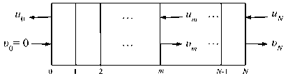
Fig. 1. Schematic of the right scattering problem for a Bragg grating: the wave is incident on the grating from the right

In the course of solving the scattering problem, it is necessary to find the spectral scattering coefficients a ( k ), b ( k ) from equations (12). The solution yields the product of transfer matrices:

a ( k ) e i ^k ^ N b ( k ) e i ^k ^ n

= T N -1 T N - 2

Calculating the matrix product (13) leads to the problem of fast polynomial multiplication, since the elements of the transfer matrices are binomials in the parameter z . Multiplying the elements of the transfer matrices yields a polynomial approximation of the spectral data: the scattering data a ( k ), b ( k ) have the form of N -th degree polynomials of the spectral parameter z .

3.    Algorithm

The numerical algorithm for solving the scattering problem finds discrete values of the spectral coefficients for N values of the wave vector k j = j A k , j = 0,1,..., N -1, with a step of A k , by calculating the matrix product for the corresponding values of the spectral parameter z j . Since the optical and spectral variables are related by the Fourier transform, the step of the discrete grid along the wave vectors A k is chosen from the condition imposed by the fast discrete Fourier transform (FFT): A k = n /(2 hN ). During the calculation of the transfer matrix products, the discretized spectra of the scattering data a ( k j ), b ( k j ), j =0, 1,…, N are determined. The desired reflection spectrum is found as the ratio of the polynomials r ( k j ) = b ( k j ) / a ( k j ). This spectrum is then used to calculate the impulse response (8) using the FFT.

The product of transfer matrices Tm of dimension 2×2, all four elements of which are binomials in the parameter z, is reduced to successive multiplication of polynomials by binomials. With each such multiplication, the degree of the polynomials will increase by one. At the m-th step of the multiplication process, for each element of the resulting matrix, the elements of the matrix of the previous step, consisting of polynomials with m + 1 coefficients, are multiplied by pairs of coefficients of the binomials. Let us estimate the total number of multiplication operations when calculating one element of the final matrix. The number of multiplications can be represented as the sum

2 ^, N = ₁¹2( ^m + 1) = 2 N ² + 2 N - 4 .

The factor 2 before the sum takes into account that for each resulting element, two products of the polynomial by the binomial are performed (two elements of the row of the matrix of the previous step are multiplied by two elements of the column of the transfer matrix). Thus, the order of the number of multiplications for one matrix element in the sequential calculation of matrix products can be qualitatively estimated as O (2 N ² ). A similar estimate O ( N ² ) for the number of operations is typical for the application of TMM to solve the direct scattering problem for Bragg gratings.

In the report [16], in the scattering problem for the system of Zakharov-Shabat equations, kindred to the Helmholtz equation, it was proposed to use the doubling strategy, the convolution theorem, and the fast Fourier transform to speed up the calculations. We will apply a similar approach here for the Helmholtz equation. The doubling strategy consists of dividing the transfer matrices into adjacent pairs during the calculation of the products. These pairs are multiplied to obtain N /2 matrices, the elements of which are second-order polynomials in the spectral parameter z . The procedure of dividing into pairs and multiplying is repeated (duplicated) until one resulting matrix remains, if the size of the discrete grid is chosen as a power of two: N =2 ^M . With each such multiplication, the degree of the resulting polynomials doubles, and the number of matrix multiplications is M – 1 = log 2 N – 1. At each m -th step, 2 ^{M – m} pairs of polynomials are multiplied, where both polynomials have degree 2 ^{m –1} and each contains 2 ^{m –1} + 1 coefficients. Direct multiplication of a pair of such polynomials requires (2 ^{m –1} + 1) ² multiplications. The total number of multiplications when calculating one element of the resulting matrix will be

2 ^ ''■ । (2 m ^{- 1} + 1) 2 2 M ^- m

= 2 2 M ^{- 1} + M 2 ^{M + 1} - 2 M - 4

And in this sum, the factor two before it takes into account that the calculation of one element of the matrix requires double multiplication of the polynomials. As a result, in order of magnitude, the duplicating calculation method gives an estimate of O (2 ^{2 M –1} ) = O ( N ² / 2). This estimate is four times smaller than in the case of sequential matrix multiplication.

The calculation of matrix products can be accelerated even more if we use the convolution theorem and the FFT to calculate polynomial multiplications. Consider the product of the polynomial f = f0+ f1z + f2z2 +…+ fjzj of degree j =2m – 1 by the polynomial g = g0+ g1z + g2z2 +…+ gjzj. This product results in a polynomial c of degree 2j =2m with coefficients ci, i =0, 1,…, 2j. The coefficients of the resulting polynomial are a discrete convolution of the coefficients of the original polynomials, provided that both polynomials are complemented with zero coefficients to degree 2j:

i

C i = X fg - 1 , i = 0,1,-,2 j .                   (14)

l =0

Direct calculation of a pair of convolutions when calculating one element of the resulting matrix will require

2 X j i + 1) = 4 j 2 + 6 j + 2

multiplications. This number can be significantly reduced by applying the convolution theorem. According to the theorem, the convolution (14) can be quickly calculated using one inverse and two forward FFTs of the arrays of coefficients of the original polynomials:

c = У ^{- l}[7 [ f ] • У[ g ]],                           (15)

where У denotes the direct FFT, У ^-1 denotes the inverse FFT, and the dot • denotes the term-wise product of the Fourier transforms of the arrays of coefficients of the polynomials f and g . An FFT of size N =2 ^M requires about O ( NM ) = O ( N log 2 N ) multiplication operations. We estimate the total number of multiplications in calculating one element of the resulting matrix using the convolution theorem, taking into account the term-wise multiplication of the results of the pair of Fourier transforms in (15). This estimate is given by the sum

2 ^ M = -i (2 m ( m + 2))2 M - m = NM 2 + 3 NM — 4 N •

As a result, for the accelerated algorithm using the convolution theorem, to calculate one element of the resulting matrix, we obtain an asymptotic estimate for the number of multiplications: O ( NM ²)= O ( N log²₂ N ).

For moderate values of M = log 2 N - 7 -13, a noticeable contribution to the number of multiplication operations is made by the term 3 N log 2 N . So, we obtained an “superfast” algorithm for calculating the spectral scattering problem, which requires only O ( N log²₂ N ) multiplication operations to calculate N spectral values of the scattering coefficients.

• 4.    Numerical simulation

The algorithm was tested using the exact solution of the Helmholtz equation for an exponentially smooth transition layer between two limiting values of the refractive index n 1 at ^ ^ - x , and n 2 at C ^ + x (see [17, 18]). The scattering potential of the transition layer – the mode coupling coefficient q ( C ) has the form of a hyperbolic secant:

• 1    dn Q . Г п ₄

q ^{( C )} = —— = —^sech —^{( C-C} c ) ,

• 2    nd C   L L L _

where C c is the optical coordinate of the layer center, L is its optical width, and the parameter Q =(–1 /2)ln( n 1 / n 2 ). For such aperiodic grating, the dependence of the refractive index on the optical coordinate C is described by the formula:

4Q         n arctan tanh[-(C-C c)]

n           2L

The dependence of the geometric coordinate x on the optical coordinate C is determined by the integral (3):

x ( C ) = £[1/ n ( C' )] d C' •

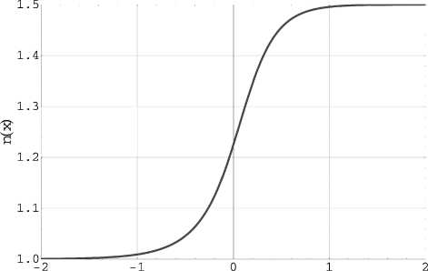
This dependence together with equation (16) describes the parametric dependence of the refractive index on the coordinate n ( x ), shown in Fig. 2.

x[/zm]

Fig. 2. Dependence of the refractive index on the geometric coordinate n(x) for the smooth transition layer, for n 1 = 1.0, n 2 = 1.5, &  = 0, and £ = 1 ^ m

The spectrum of the reflection coefficient for the grating is given by:

Q r(d+ )Г(f- )Г(f+) r(k) =,

’ п Г ( d - ) Г ( g - ) Г ( g + )

where Г is Euler’s gamma function, and

• , 1 i k L   J 1i

• d + = — +--, d - =,

2 п 2 п

.

• .f.=1 - i^ ± ®, g.=1 ± ® 2 п пп

Calculations of the direct scattering problem for the Helmholtz equation were performed with the following set of parameters: wavelength X = 1 цш, refractive indices of the layer n 1 = 1, n 2 = 1.5, the central coordinate C c = 0, and the optical with L =1 цш. The calculation interval was chosen so that the mode coupling coefficient q ( C ) at the interval edges approached zero with high accuracy.

Numerical simulations using the accelerated algorithm and comparisons with the exact solution showed that when the grid size N was doubled, the rootmean-square error norm of the reflection coefficient calculation decreased by a factor of four, indicating that the calculation accuracy was of the second order. For instance, the Euclidean norms ε of the absolute error in calculating the reflection coefficient were ε =0.000041082 for N =211 and ε =0.0000102715 for N = 212. The error ratio was 3.9996.

Fig. 3 shows the graph of the computation time Time (in microseconds) of the algotithm, divided by the asymptotics N log²₂ N as a function of the degree M = log 2 N , for integer M = 8, 9,…, 17. It is evident from the figure that for M > 14 the computation time begins to correspond to the asymptotics, since their ratio becomes constant.

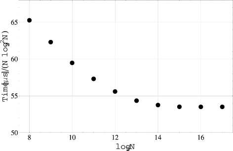
Fig. 3. Graph of the algorithm running time Time (in microseconds) divided by to the asymptotics N log²₂ N depending on the factor log 2 N

Conclusion

In this study, we addressed the problem of calculating the spectra of aperiodic Bragg gratings by solving the direct scattering problem for the Helmholtz equation. An accelerated algorithm was proposed, which requires asymptotically about O ( N log²₂ N ) arithmetic operations (multiplications) for a discrete grid of size N . This algorithm uses an integral approach to discretization and demonstrates second-order accuracy for smooth, localized solutions of the direct scattering problem. It approximates the polynomial dependence of spectral data (scattering coefficients) a ( k ), b ( k ) on the spectral parameter z = exp(4 ikh ), which determines the reflectivity coefficient r ( k ). The algorithm leverages the duplication strategy, the convolution theorem, and the fast Fourier transform to achieve high efficiency. Numerical simulations using the comparisons with the exact solution confirmed the algorithm’s second-order accuracy and its high computational speed, in accordance with the estimates obtained. Finally, we note that the applicability range of the proposed algorithm is limited to onedimensional scattering problems and dielectric media in which attenuation can be neglected.

Acknowledgments