Accelerating Cross-correlation Applications via Parallel Computing

Distributed computing is a science which solves a large problem by giving small parts of the problem to many computers to solve and then combining the solutions for the parts into a solution for the problem. Grid computing (or the use of a computational grid) is applying the resources of many computers in a network to a single problem at the same time. “Distributed” or “grid” computing in general is a special type of parallel computing that relies on complete computers (with onboard CPUs, storage, power supplies, network interfaces, etc.) connected to a network (private, public or the Internet) by a conventional network interface, such as Ethernet. Modern Operating Systems (OSs) today are aware of multiple CPU cores and can automatically manage parallel processes and send each to run using a different core, allowing effective parallelization.

First step in parallel programming is the design of a parallel algorithm or program for a given application problem. The design starts with the decomposition of the computations of an application into several parts, called tasks, which can be computed in parallel on the cores or processors of the parallel hardware. The decomposition into tasks can be complicated and laborious, since there are usually many different possibilities of decomposition for the same application algorithm. The size of tasks (e.g., in terms of the number of instructions) is called granularity and there is typically the possibility of choosing tasks of different sizes. Defining the tasks of an application appropriately is one of the main intellectual works in the development of a parallel program and is difficult to automate.

With distributed computing, an initiator machine sends processes for parallel execution on other machines connected to the network. These processes will then run on these machines alongside any other processes running at the time on the OS, but will run in a special self-contained virtual environment that completely emulates the initiator's environment, including installed applications, file system, registry, and environment. An important issue of such systems is the efficient assignment of tasks and utilization of resources, commonly referred to as load balancing problem. Load balancing algorithms can be classified into two categories: static or dynamic. In static algorithms, the decisions related to load balance are made at compile time when resource requirements are estimated. A multicomputer with dynamic load balancing allocate/reallocate resources at runtime based on no a priori task information, which may determine when and whose tasks can be migrated. While machines in a cluster do not have to be symmetric, load balancing is more difficult if they are not.

The aim of this paper is to study the possibility of accelerating the cross-correlation application through decomposing its computations into several parts and distribute these parts among the reachable computers over the network. After finishing execution of these parts the results are returned to the main caller program.

• II.    BACKGROUND

A.    Distributed Computing

Distributed computing is a type of computing that deals with applications that run simultaneously on distributed systems that communicate through computer network in order to solve massive computational problems. Tanenbaum and Steen have defined a distributed system as “a collection of independent computers that appears to its users as a single coherent system” [1]. The main driving force for the development of distributed computing is the requirement for high-performance computing resources for solving massive scientific computational problems, which led to the idea of dividing the problems into smaller tasks to be processed in parallel across multiple computers [2]. The development of computing and high-speed network infrastructures in the past few years has also made it possible for distributed computing systems to provide a coordinated and reliable access to high performance computational resources.

Distributed computing can be classified broadly into types. The first is high-performance computing on parallel heavy-duty systems that provide access to large-scale computational resource and are common for computationally intensive applications. These resources involve high investment cost and are usually limited at few institutions and research centers. Another distributed computing solution is that is becoming increasingly popular recently is to perform computations on clusters of low-cost commodity computers connected over high speed network. The advances in high-speed network communications and its inexpensive availability made this trend more practical over expensive parallel supercomputers.

The parallel execution time is the time elapsed between the start of the application on the first processor and the end of the execution of the application on all processors. This time is influenced by the distribution of work to processors or cores, the time for information exchange or synchronization, and idle times in which a processor cannot do anything useful but wait for an event to happen. In general, a smaller parallel execution time results when the work load is assigned equally to processors or cores, which is called load balancing, and when the overhead for information exchange, synchronization, and idle times is small. Finding a specific scheduling and mapping strategy which leads to a good load balance and a small overhead is often difficult because of many interactions.

B.    NET Remoting API

The .NET Remoting API is the equivalent of the Java Remote Method Invocation (RMI) API. Both frameworks allow objects on a client machine to communicate with remote objects on a server. The infrastructure required in .NET appears simpler than in Java’s RMI. What makes Remoting (or equivalently RMI) so attractive is that the low-level socket protocol that the programmer must normally manage is abstracted out. The programmer is able to operate at a much higher and simpler level of abstraction. In both languages there is some overhead in the form of boilerplate protocols that must be observed in order to setup the handshaking between the client and server machines. Once this is done, sending a message from a client machine to a server object uses the same syntax as sending a message to a local object. The metaphor of object-oriented programming remains central to this distributed programming [4].

Considering MSDN, .NET remoting enables building widely distributed applications easily, whether application components are all on one computer or spread out across the entire world. It allows to build client applications that use objects in other processes on the same computer or on any other computer that is reachable over its network. According to this sort of technology, a simple shape of grid computing with one manager and some executers connected to the manager is shown in Fig. 1.

Figure 1 : Grid computing in LAN

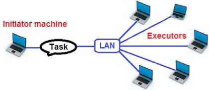
The initiator machine (manager) decomposes the computations of the application into several parts, called tasks. The manager invokes these tasks as methods to the executers on the remote computers. The executer is a Windows service program, which in turn compiles the code and executes the created assembly. After finishing executing the method, the executer invokes a manager's method and sends the results back to it.

C.    Cross-correlation

Cross correlation [5-7] is a standard method of estimating the degree to which two series are correlated. In signal processing, cross-correlation is a measure of similarity of two waveforms as a function of a time-lag applied to one of them. It is commonly used for searching a long-signal for a shorter, known feature. It also has applications in pattern recognition, single particle analysis, electron tomographic averaging, cryptanalysis, and neurophysiology. For continuous two 1-D analog signals f and g functions, the crosscorrelation is defined as:

ю c (t) = (f * g )(t) deft f (t) g (t + т ) dT -Of

Where denotes the cross-correlation lag. Similarly, for discrete functions, the cross-correlation is defined as :

⁽. f * g ) [ n ] def S 2₌_„ f [ m ] g [ n + m ]

The normalized form of cross correlation r at delay d between two series                   is defined as:

rd

Z , -[ ( x ^[ i ^]- x ) * ( У ^[ i - ^{d ]-} У ) ] V S i ( x ^{[ 1 ]-} x ) 2 V ^ i ( y ^{[ 1} - ^{d ]-} y ) 2

and and are the means of the corresponding series. The coefficient, r, is a measurement of the size and direction of the linear relationship between variables x and y. If these variables move together, where they both rise at an identical rate, then r = +1. If the other variable does not budge, then r = 0. If the other variable falls at an identical rate, then r = -1. If r is greater than zero, we have positive correlation. If r is less than zero, we have negative correlation. The sample non-normalized crosscorrelation of two input signals requires that r be computed by a sample-shift (time-shifting) along one of the input signals. For the numerator, this is called a sliding dot product or sliding inner product.

If the above is computed for all delays d=0,1,2,...N-1 then it results in a cross correlation series of twice the length as the original series.

Cache, 1.50 GHz), 2 GB RAM.

• -    Sony VAIO, VGN-CS26M, Intel^® Core^™2 Duo Processor P8600 (2.40 GHz), 3 GB RAM.

• -    Lenovo with Intel® Core™ i7 CPU L620 @ 2.00 GHz, installed memory (RAM): 4 GB.

Operating system: Windows 7.

The algorith m of the cross-correlation is shown in

List-1:

List-1:

z , [ ( x и- x ) * ( y i ' - d ] - y ), _

Z- JL ( y i ' - d ] - y 1

// compute the following cross-correlation function

Z.( x И^- x ) * ( y ^l ' ^- d ^{] -} y )

// r ⁽ d ) =

L ( x [ ' ] - x ) ^ , ( y [ , - d ] - y )

There is the issue of what to do when the index into the series is less than 0 or greater than or equal to the number of points. ( -d < 0 or -d >= N) The most common approaches are to either ignore these points or assuming the series x and y are zero for < 0 and >= N . In many signal processing applications the series is assumed to be circular in which case the out of range indexes are "wrapped" back within range, i.e: x(-1) = x(N-1), x(N+5) = x(5) etc.

• III.    EXPERIMENTAL MEASUREMENTS AND RESULTS ANALYSIS

This section is dedicated to present and analyze performance measurements of the following three implementations:

- Running the cross-correlation algorithm as a standalone application on different three independent platforms (different hardware and operating systems). The times of processing t1, t2 and t3 are recorded for the three platforms respectively.

- Modify the cross-correlation computing application to be distributed and performed simultaneously on the prescribed three different platforms. The computing procedure will be partitioned equally and invoked remotely to the three platforms.

- Modify the last application once again to address the load balancing problem; the computing procedure will be partitioned to different three pieces. The size partitioning ratios are proportional inversely with the times of processing of the three platforms (t1, t2 and t3).

A.  Standalone Implementat on

The machines used to perform the benchmarking were:

- FUJITSU Intel® Celeron® Processor B800 (2M as following:

generate_signal(x);

generate_signal(y);

compute  = mean_value of signal_x;

compute  = mean_value of signal_y;

//compute the denominator denom =

“   JX(xi']-X)2 -jПyi'-d]-y)7    as following for (i = 0; i < length_of_signal; i++)

{ sx += (x[i] - ) ^2

sy += (y[i] -   ) ^2

// perform the cross-correlation

//Compute r ( d ) =

^J [ (. ^x l ' ] -. ^x ) * ( y l £ - d ] -. y ) ]

denom as:

for (delay = -maxdelay; delay < maxdelay; delay++) { sxy = 0;

for ( i = 0; i < length_of_signal; i++)

{

• j = i + delay;

if (j < 0 || j >= length_of_signal)

continue;

• ^{e s}s^exy += (x[i] - ) * (y[j] - );

}

r[d] = sxy / denom;

d++;

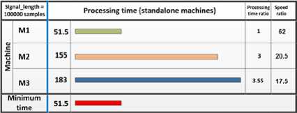
Figure 2: Algorithm processing at standalone machines

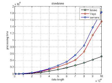
Figure 3 : Comparing time of processing for different data lengths at standalone machines

The algorithm is performed for the two signals x[], y[] having the same length. The processing times have been recorded as in Fig.2, Fig.3. The figures compare the performance of the three platforms when executing the same prescribed cross-correlation algorithm.

B.    Uniform Partitioned Cross-Correlation

One issue that can complicate development efforts in building a parallel computing architecture is the application's suitability for "slicing" into multiple, independently executable parts that can run in parallel. The algorith m prescribed in list-1 has been modified and uniformly partitioned to be run remotely on the same three machines. The “length_of_signal” is divided equally into three parts between the three machines:

part_size = (int)(length_of_signal / (no_of_pcs));

where “no_of_pcs” is number of machines. For the first machine, the cross_correlation loop starts from location=0 for size = part_size. For the second machine, the loop starts from location = part_size for size = part_size. For the last machine, the loop starts from location = 2*part_size for size = part_size.

List-2:

// Assign and send part of the cross-correlation to each // machine in the local area network.

for (delay = -maxdelay + location; delay < - maxdelay + location + part_size; delay++)

{ double sxy = 0;

for (i = 0; i < length_of_signal; i++)

{ j = i + delay;

if (j < 0 || j >= length_of_signal)

continue;

else sxy += (x5[i, 1] - mx) * (y5[j, 1] - my);

}

r[d] = sxy / denom;

d++;

}

// upon completing the dedicated part of the crosscorrelation

// procedure on a certain machine, the returned results are

// placed in the correct place of the main output array.

Fig.4, Fig.5 compare the performance of the three platforms when executing the assigned part of the crosscorrelation algorithm (list-2). It can be noticed that each machine finishes the execution of the assigned part at different time. The overall processing time is the higher time:

overall_processing time = max (machine_time1, machine_time2, machine_time3).

Where    machine_time 1, machine_time2 and machine_time3 are the processing times at machines m1, m2 and m3 respectively.

Choosing signal of length = 10 x 104 samples as a comparison case, the processing times at m1, m2 and m3 machines are 18, 35 and 50 seconds respectively. Accordingly, the overall processing time = max(18, 35, 50) = 50 seconds. Inspecting Fig.2, the signal with the same length (10 x 104 samples) needs 51.5, 155 and 183 seconds to be completed separately on machine m1, m2 and m3 respectively.

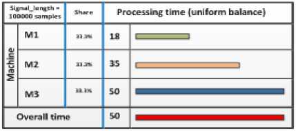
Figure 4: Algorithm processing remotely with equal loads

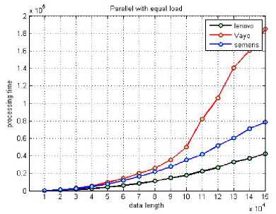
Figure 5 : Comparing time of processing for different data lengths remotely with equal load

C.    Balanced Load Grid-computing Implementation

The algorithm prescribed in List-2 has been further modified. The algorithm, in its new form, distributes the cross-correlation processing load between the available remote PCs in the LAN. The load is distributed according the speed of each PC’s processor depending on the results obtained in List-1:

Assuming that the same task of load L has executed on n computers PC1, PC2, PC3,…., and PCn, yielding to processing times T1, T2,.., …, and Tn respectively. Accordingly, the ratio between the corresponding speeds S1, S2, …. , and Sn can be computed as:

	LL	L
s 1: s 2:	... ^            :       : n    T 1 T 2 11	...                                 (1) n 1
s 1: s 2:	... 5        :       : n    T 1 T 2	... T                         (2) n

Now, assume the task L is to be partitioned over the computers PC 1 , PC 2 , PC 3 , …. , and PC_n . The goal is to find the share L i of each computer such that:

L = L1 + L2 + ... + Ln , and(3)

The time of processing at PC_i is and the overall time T = max ( ). It is desirable to minimize T such that:

ti = 12 = ...:= tn(4)

The ratio between loads is:

Li: L 2:...: L = ti ^i: 12 S2:...t„S„(5)

From 2, 4 and 5:

L ₁: L ₂

L ₁: L ₂

L L

T ₁ T ₂

T

n tL .nT n

locations[i] = current_location;

current_location = current_location + sizes[i];

}

Then, the task is invoked to each PC and both the part_size and location are passed as parameters.

// Assign and send part of the cross-correlation to each // machine in the local area network.

for (delay = -maxdelay + location; delay < - maxdelay + location + part_size; delay++)

{ double sxy = 0;

for (i = 0; i < length_of_signal; i++)

{ j = i + delay;

if (j < 0 || j >= length_of_signal) continue;

else sxy += (x5[i, 1] - mx) * (y5[j, 1] - my);

}

r[d] = sxy / denom;

d++;

}

// upon completing the dedicated part of the crosscorrelation

// procedure on a certain machine, the returned results are

// placed in the correct place of the main output array.

Fig.6, Fig.7 demonstrate the times of processing for different signals lengths. It is clear that the processing at the different platforms had been completed almost at the same time. Also, for the signal length of 10x104 the overall time has been reduced to 35 seconds compared to 50 seconds when performing the same task but with distributing it equally on the same platforms (section List-2).

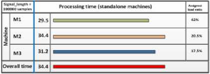
Figure 6: Algorithm processing remotely with balanced loads

Consequently, to achieve minimum time of processing the total load L should be partitioned between the available PCs in the same ratio of times of processing when the same load L is executed separately on each PC. The above described algorithm is practically implemented as following:

List-3:

//to determine the size and start position of every part int current location = 0;

for (i = 0; i < no_of_pcs; i++)

{ sizes[i] = ( length_of_signal * ratios[i] / 100);

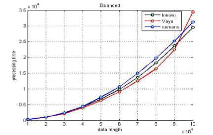
Figure 7: Comparing time of processing for different data lengths remotely with balanced loads

• IV.  CONCLUSION

The cross-correlation computing algorithm has been executed using three different scenarios. In the first one, the algorithm has been executed separately on three different hardware platforms using different signal lengths as test data. The processing times obtained from this scenario has been used as a reference for comparison in the other two scenarios. In the second scenario, the same algorithm has been partitioned into three equal parts and invoked remotely to the same platforms to be executed there. The results are gathered upon finishing the execution of the three processes. The overall time was greater than that obtained in the first scenario because some processes will finish while others still busy. In the last scenario, the times of processing obtained from the first scenario have been used as a guide to determine the size of each algorithm partition. These partitions have been invoked remotely to the same platforms to be executed there. The overall time has been greatly reduced compared with the overall time obtained from the other two scenarios. The end result is the successful implementation of the cross-correlation algorithm on a distributed environment which demonstrates the possibility of performing more complex computational problems within minimum time.