Accelerating the Response of Query in Semantic Web

Author: Nooshin Azimi, Shahla Kiani
Journal: International Journal of Computer Network and Information Security(IJCNIS) @ijcnis
Article in issue: 8 vol.6, 2014.
Free access
Today, XML has become one of the important formats of saving and exchanging data. XML structure flexibility enhances its use, and the content of XML documents is increasing constantly. As a result, since file management system is not able to manage such content of data, managing XML documents requires a comprehensive management system. With the striking growth of such databases, the necessity of accelerating the implementing operation of queries is felt. In this paper, we are searching for a method that has required ability for a large set of queries; the method that would access fewer nodes and would get the answer through a shorter period of time, compared to similar ways; the method which has the ability of matching with similar ways indicator, and can use them to accelerate the queries. We are seeking a method which is able to jump over the useless nodes and produces intermediate data, as compared to similar ones. A method by which nodes processing are not performed directly and automatically through a pattern matching guide.
Query, Semantic Web, Optimization, XML Structure
Short address: https://sciup.org/15011328
IDR: 15011328
Text of the scientific article Accelerating the Response of Query in Semantic Web
Published Online July 2014 in MECS
Since in XML world, a standard method such as SQL in relational databases has not been achieved yet, the effectiveness improvement of XML queries still goes on. There are many methods introduced about this field that we will show their most important objections, below [1].
-
1. Production of intermediate data (data that are produced only for user response and have no more applications)
-
2. Increasing the query response by increasing
-
3. Involving all query nodes for achieving the
-
4. using for a small group of the queries and operators.
-
5. No compatibility with the methods that are used to index the document.
query length.
response.
Many researchers also have tried to apply the traditional methods of relations for managing XML documents, but the structure of an XML document into a tree format is different from the relation and old structure. . As an instance, in a relation model, the table data are on a same level and relations between tables as links can be set up too. But there are other relations in a XML document such as parental – filial, ancestral – racial and sibling. Thus the complexity of user queries is more than before, and the responses ranges have been altered. On the other hand, applying of the simple operators such as NOT is not possible readily as before. Thus providing a method for this different structure should have the following capabilities.
V The ability of responding to the queries at the shortest possible period of time.
V The Same performance for all existing queries in XML
V No need to long preparing of the document.
V Compatibility with all existing indexes.
V No production of the useless data.
V The existence of the linkage between the response and the query
This paper is organized as follows. In the next section, the research background to respond queries to achieve all existing nodes in the document is presented. In this section, advantages and disadvantages of a method called TJFast [3], is expressed.
The following section includes discussion on the problems and its dependency on other parameters is presented.
Next section the general structure of the provided algorithm is presented and and then present an exact explanation of all steps.
Other section is explained the application of index table in complex queries
Then, our algorithm is evaluated and compared with a similar algorithm in the next section.
Finally, the paper is concluded with highlights of an open issue.
-
II. The research background
Up to now, many methods have been proposed for this task, including:
-
• Nested loops
-
• STRUCTURAL JOIN
-
• Staircase
-
• HOLISTIC TWIG JOIN
-
• JFAST
Q1: STUDENT//BOOK [TITLE=’XML’];
This method numbers the tree as decimal or coded Dewey [11] [12].
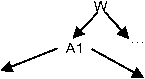
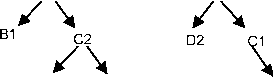
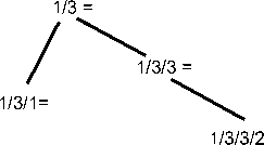
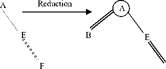
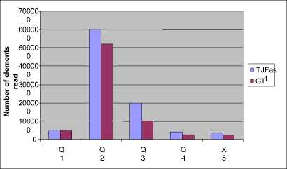
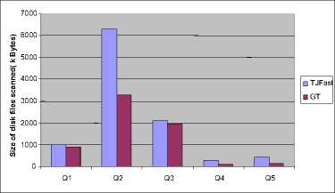
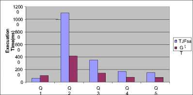
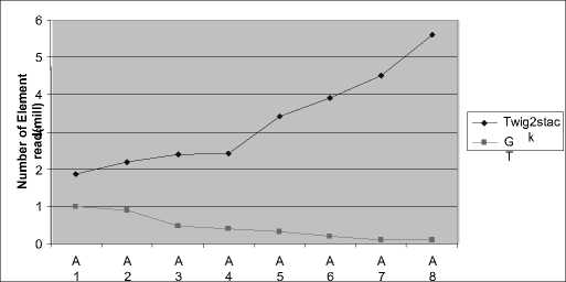
Using this atamata, TJFast firstly decodes internal nodes, and then compares them to get the response. TJFast compares only the query leaf nodes, thus the number of achieved nodes in this method will be much fewer than the same methods. For example, we just need to consider n member for a query of n branch with m members where n< V In many cases, the time and content of FST is significant and applying it is not economical. V TJFast takes a long time for decoding the nodes and this makes the total time more than the times in the same methods. III. Defining the Problem As we observed in the previous section, processing XML queries still needs to be improved. Lack of effectiveness in this field made many of the users not to accept XML as a data, and again insist on the rational method. Given the deficiencies of the existing methods, we need a plan that has the capability to meet the following objectives: V Having the requirement of the minimum nodes to respond the queries. V Getting the minimum interface or intermediate data content – the data that are not a part of the final respond, and are used just to produce the final respond. V Getting the minimum useless data content - the data that are not as a part of the final respond, and are processed unreasonably. V Not to compare nodes directly, and being capable of combining with Path Index [6] methods. IV. The General Structure Of The Provided Algorithm Step 1: In this step, query as Path index methods is firstly performed on SS, Here; the query is not performed as its primary and complex leaf, but it is broken into several single branch queries that are responded in all path index methods [7]. Then all the single branch queries are performed on SS separately. The main purpose of this step is reducing the range of the nods searching. SS is used as the pattern matching guide. Step 2: All the single-branch queries are performed on SS separately, and each is set to return as the respond. Note that these are the nodes on SS, not the ones on the actual document. Step 3: The document is numbered at Dewy encoding. As presented in the previous chapter, the nodes related to each group SS node are arranged at Dewy in its Extend. Now third step of the query performs similar to Containment join. Here, query leaf nodes which are in Extend are compared considering IT, and the final respond is produced. A. The query guide Basically, the query guide is like a document schema. SS is much related to DTD or a document XML Schema [2]. A document schema shows the structure and general relationship among the elements, and is very little related to the content and size of the document data. Its structure and is typically steady or has a little change. But this SS in XML world can be made in different ways. For example, in SS, [4] [5] [6] [7] [8] [9] [10] are produced through different methods, and each has its special quality and trait. Fortunately, the following criteria about SS have been proved during the recent years. V SS content is much smaller than the actual document data content. For example, the known dataset, Treebank [11], Xmark [5], DBLP [4]. That has the sizes of 130,897 and 532 Mb, respectively; their schematic contents are 2.8, 4.2, and 3 kb. V A document SS has a poor relationship with the data size in the document. B. Continous Model In the XML world, SS can be made through different ways. For example, SS is produced by different methods that each has its special quality and trait. Thus, there are many Path indexes to be chosen, but each one of them tries to respond to complex queries by itself. So many of the queries require achieving the actual document data, and as a result, they are not useful enough. Since the Path index we choose for our plan is just to look for SS and to respond to single branch queries, they should have only two following characteristics: V Its SS should be small and respond single branch queries promptly. V It should be useful for all possible (*,?, / /) operators for single branch queries. Among all Path indexes, the best option that provides only two items above is YAPI [5] that is the fastest and cheapest for responding to a single branch queries. C. First step: Performing Single Branch Queries on the Pattern Matching Guide As stated before, we should break the query. This breakage is performed so that the query breaks into the single branch queries. Then each single branch query is separately performed on SS. Fortunately, in most of Path index methods, from SS and with no need to achieve document data, single branch queries are simply able to be responded. In this step, we compare all single branch queries with the document SS, and since the document is encoded of Dewey, and the lower nodes have some heterogeneous information from their upper nodes (the covered path from the root), keeping and achieving the query leaves for each branch will only be required. The result of this performance will be getting a list of points in SS for each single branch query. The points address will be absolutely (from the root to the node). D. Second step: Index Table Production The primary definition of the index table: It's a three-column table that the first two columns of the leaf nodes of each branch in SS and its third column is the point level of the connection between two nodes. So, every record of this table shows a task called the Corresponding Act. After that in the first step, the query is converted into the single branch queries, and the leaf nodes of the single branch queries in SS are achieved; now we should get the connection point level among the leaves. The result of the single branch query performances on SS is finding a list of the nodes for each single branch query. These points’ addresses are absolute, not relative. It means each node address of the tree root is completely certain. Now, to get the connection point level among the branches, we select a node from the list of each branch leaf, and compare their paths. If the selected nodes paths are equal from the root to the query connection point level, we add those two nodes with the connection point level to IT. Fig 2: A sample of index table The primary algorithm of IT production for a two-branch query is as follows. This is a quasi-code and is just for two-branch queries. This algorithm for complex queries is as follows. Input: Q as TPQ Output: IT as Index Table A2 B2 A3 D1 D3 Fig 1: Assumed SS for examples 1: Let A and B the two leaves of Q A and B are two nodes of the query leaf. 2: Let JP = Joint point between A and B The connection point level shows the connection node of two branches. 3: Let AL = list of SS nodes match A branch 4: Let BL = list of SS nodes match B branch AL and BL show the Extend lists of A and B nodes, respectively. These nodes are the found leaf nodes for each branch of the query. 5: for each an ∈AL do 6: for each bn ∈BL do 7: for each JP1 in an, JP2 in bn do 8: if an.Prefix(JP1) = bn.prefix(JP2) then 9: IT.addREC(an, bn, JP1.level)) 10: end if 11: end for 12: end for 13: end for The lines perform the binary comparison of the nodes. Note that, a record may be added to the result table for each connection point level. If each compared two has a similar prefix to the connection point level, a record which was made from two nodes and the connection point level between them is added. E. Step Three: The Production of the Final Results The final results are produced considering the result table. Each record of the table guides the query processor to get a part of the response. The set of these parts produces the final response. Therefore, final results are the set of the returned results by each record. The procedure of step 3: Each record of the index table has three fields. The two first columns are two nodes in SS, and the third column is the connection point level between two nodes. As observed in figure 3, the actual document nodes are ordered toward their Dewey code in Extends. Now, the Extend lists of both nodes in SS should be compared with one another. If the prefix of the compared two nodes are equal to the connection point level (the third field), both are related to the response. This procedure is continued until one of two lists ends. This is called the Corresponding Process. This array shows the list of the external nodes. 1: Let L1= ET.field1.extend 2: Let L2= ET.field2.extend L1 and L2 show the list of the Extends of the two nodes which should be compared with one another. 3: Let node1= first node of L1 4: Let node2= first node of L2 These two moves like two pointers along Extend list of the two nodes. 5: Let L= ET.field3 // level of JP L shows the third field of the table or the connection point level. This is just the level that the elements of two lists should be compared with one another. 6: while (one of L1 or L2 reach the end) do 7: for each a in L1, b in L2 that 8: a. prefix(L) = prefix(L) then 9: (a, b) add to output Lines 8 and 9 show the nodes which are equal to the connection point level and will be from the corresponding process respond. It means that they have had a successful corresponding process. 10 else if node1.prefix (L) > node2.prefix (L) then 11: node2= L2.Next () 12 else 13: node1= L1.Next () Lines 11 and 13 show the nodes which haven’t had a successful corresponding process. For the nodes that are equal to no nodes to this level, the smaller node courser should prepare the next element for processing. 14: end if 15: end for 16: end while Fig 3: A sample of TPQ in document Algorithm_1: Final Index-Proc The quasi-code of the final production is as follows. The lines 8 and 9 show the nodes which are equal to the connection point level and will be related to the corresponding process respond. For nodes that are equal with no nodes to this level, next node should be processed. Pay attention to the term next( ). Input: ET as record of Index Table ET is the guidance table. Output: Output list as array of matched nodes V. The Application of Index Table in Complex Queries The general process of algorithm to response to a multi-branch query was stated through the previous section, but there are more complex queries in XML structure. Through this section, the flexibility and application of the index table to response these queries are studies so that once processing the query leaf nodes, the response is resulted. A. Connection Points with More than Two Branches As the index table is primarily defined, IT indicates a three-column table in which the first two columns show each branch nodes and the third column show interface between them; but in queries world, there might be several branches connected at a point. Consider Q2 as an example: Q2= //A [. /C][. /D] / B; This is a three-branch query in which three branches of B, C and D are connected at a point, i.e. A. here; it's just need to change the definition of IT as follows. The second definition of the index table: IT is a table with M+1 columns for connecting to a connection point having M sub-branches tin which columns first to M are the branches leaves and the last column will be the interface among all nodes. Algorithm_2: Final Index-Proc On the other hand, to produce the ultimate response to each IT cord, the figure pseudo code need to be changed into the following pseudo code, since in this case, the numbers of the compared lists are more than two. LET A1, A2… An = field1, field2… fieldn These are Extend lists that should be compared with each other. The last field shows the common connection point among the compared nodes. For each a1∈A1, a2∈A2, …. , .an∈An do These lines compares the list elements with each other, and they will be the component of the ultimate response only if all have a same prefix within this level. Else Min(a1,a2,…an).Next() But for each unsuccessful correspondence, the smallest element is required to move to the next node. Endif Endfor B. Queries with more than two connection point As observed in the previous section, the most important state occurred for our queries were a mode we had to study the existence of a number of branches simultaneously. We must look for a point called the connection point. A connection point is a node in TPQ in which several query branches are connected. In one query, each IT is used for one connection point. Thus, for the queries with m number of connection point, m number of IT is needed. But these ITs can't act independently, and there is dependence among them. So we need two changes. The first change: In the previous figure, IT model should be used instead of one IT. The definition of IT Model: A set of n number of IT for a query with n number of connection point that shows the relation among them. As an example, suppose we want to make IT Model for the figure below. The method is that we find three singlebranches A//B/C, A//B/D and A/E//F from sample accordance guide. There is a connection point called B for the two branches A//B/C and A//B/D. After solving this part of query – when conditional bs as the connection point are found – now, the connection points among the branches A//B and A/E//F should be found. Another connection point is A which is the connection point between two first branches and the third branch. As you observe in the following figure, the connection point A uses the exit of the connection point B. as a result; ITB exit is used as one of ITA fields. B A C C D RTB D F C D Fig 4: The process of the omission of the Multi-branch queries complexity F Fig 5: BRTB F An exam ple ofB RTA The second Change: that should be done in order of the nodes processing for making Index. This changing is shown in the following pseudo-code. Algorithm_3: Final Index-Proc 1: Assume Order process in It_Model is: 2: IT1^IT2^„^ITn 3: Match _ Proc(IT1,1) The above pseude-code acts bottom-up which mean it firstly processes the connection points in the lower location in TPQ tree.The procedure is done so that it starts the process from the first IT when there is aprocessing (relation) order among several ITs (line 3).A recessive procedure called Match_Proc is used in order to follow the processing order. 4: Match_Proc(ITi,i ) 5: If (i=n+1 ) then 6: Successful match This trend goes on as far as matching would be successful for all ITs (line 5 and 6). 7: Elseif (Match_Proc in ITi IS Successful) then 8: Match_Proc (ITi+1, I+1) This procedure acts when there is a successful match in an IT (line7), the process is tested for the next IT (line 8). 9: Els 10: Min (ITi, ITi-1).Next () 11: Match_Proc (ITi-1, i-1) When there is an unsuccessful matching, Cursor movement should be done in one of two ITs, either the present or the previous one (Line 10); and matching begins again from the previous IT (Line 11). 12: EndIf 13: EndProc VI .The Simulation Field and the Comparison Criteria The selected data set: four data set called Treebank, DBLP, Xmark are used to test guide table method. Each one of data set in XML world is known for the researchers in this field, and most of the methods are tested on the same data. These documents require the pattern production for the first query performance. For these documents, it should be surveyed once to get the pattern tree schema. All three documents characteristics are represented totally in table (1). Table I. Characteristics of known data sets XMark DBLP Treebank Data size(MB) 582 130 82 Nodes(million) 8 3.3 2.4 Max/Avg depth 12/5 6/2.9 36/7.8 The Random Data Set (RDS): In addition to the known and considered documents, the random data set are produced to perform the queries, so that the guide table method in this kind of the document is shown too. The way of the set production is that a pattern is randomly made with the depth 12 and maximum 10 children. The elements labels of this graph are only the letters a,b,c,d,e and f. Table II. Characteristics of randomized data sets Dataset name Data size(MB) Node(million) Depth Random dataset 890 8.3 12 Hardware: All data are performed on a system with a processor of 202GHz and a processor of Intel Pentium IV on windows XP or with 2GB of main memory. A. The Comparison with Similar Methods and Providing Statistic Results The experimental data are presented during three steps. First step of the comparison is the guide table method with the similar ways, TJFast and Twig2Stack. In this step, the method efficiency is represented rather than similar ways. In the second step, the way efficiency has come to jump over the useful nodes. Five queries of the table 3, that each one has its own characteristic have been tested on both TJFast method and the guide table. Table III.Queries running on RT and TJFast Query Name Query Database Q1 /site/people/person/gender XMARK Q2 /S[.//VP/IN]//NP Treebank Q3 /S/VP/PP[IN]/NP/VBN Treebank Q4 //article[.//sup]//title//sub DBLP Q5 //in proceedings//title[.//i]//sup DBLP Fig 6: Number of used nodes Used main memory size: Considering figure 6, the used main memory size for the query respond in guide table is less than TJFast method. In TJFast method, when two nodes are compared with one another, some nodes require to be saved, because they may produce a part of the respond by being compared with another node. Since TJFast by automatically direct comparing the nodes tries to reach the query respond. Fig 7: Used space in main memory Performance time: as observes in figure 7, TJFast performance time is far more than guide table time, for TJFast requires decoding for each internal data, and this wastes a long time for each node: As it's clear in QI, guide table method has no difference with TJFast. Its reason refers to being single branch of the query that requires no comparison in document. Only proper leaves are enough for finding the location. Fig 8: Performance time Fig 9: Single branch queries VII . Conclusion As previously noted, XML is one of the most important issues of saving and exchanging data. Flexibility of XML structure enhances its use consequently the content of XML documents is increasing. This paper proposed a novel method that would access fewer nodes and would get the answer through a shorter time, compared to similar ways. In addition, this method is able to jump over the useless nodes and produces intermediate data, as compared to similar ones.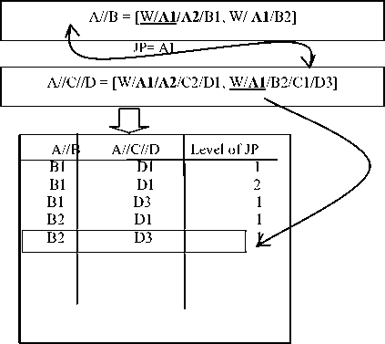


References Accelerating the Response of Query in Semantic Web
- Sayyed Kamyar Izadi, Mostafa S. Haghjoo, Theo H¨arder,” S3: Processing tree-pattern XML queries with all logical operators, Data & Knowledge Engineering “Volume 72, Pages 31-62. (2011), doi: 10.1016/j.datak.2011.09.003.
- SangKeun Lee, Byung-Gul Ryu, Kun-Lung Wu, Examining the impact of data-access cost on XML twig pattern matching Original Research Article Information Sciences”. , Volume 203, Pages 24-43, October 2012.
- Chung, C., Min, J., Shim, K. Apex:" An adaptive path index for xml data.", In Proc ACM Conference on Management of Data SIGMOD: 121 - 132(2005).
- Cooper. B., Sample. N., Franklin. M., Hjaltason. G., Shadmon. M. A Fast Index for Semistructed Data, In Proc. 14th VLDB conference: 341 – 350(2008).
- R. Kaushik, P. Shenoy, P. Bohannon, and E. Gudes."Exploiting Local Similarity for Indexing Paths in Graph-Structured Data". In IEEE/ICDE, pages 129--140, San Jose, California, 2009.
- Kaushik. R., Bohannon. P., Naughton J. and Korth. H, Covering Indexes for Branching Path Queries, In Proc. 11rd SIGMOD Conference: 133 – 144(2010).
- Kaushik. R., Krishnamurthy. R., Naughton. J., and Ramakrishna. R. On the integration of structure indexes and inverted lists, In Proc SIGMOD Conference: 779 - 790 (2009).
- Fouad, K., Harb, H. & Nagdy, N. (2011). Semantic Web supporting Adaptive E-Learning to build and represent Learner Model. The Second International Conference of E-learning and Distance Education (eLi 2011) – Riyadh.
- Milo T., and Suciu D.., Index Structures for Path Expressions. In Proc. 7th .ICDT: 277 - 295(2008).
- Yiqun Chen,Jinyin Cao,” TakeXIR:a Type-Ahead Keyword Search Xml Information Retrieval System”,(IJEME) International Journal of Intelligent Systems and Applications ,Vol. 2, No. 8, August 2012.
- Dewey. M. Dewey Decimal Classification System. http://www.mtsu.edu/~vvesper/dewey.html.
- O’Neil. P. E., Pal. S., Cseri. I., Schaller. G., Westbury. N., ORDPATHs: “Insert Friendly XML Node Labels.”, In Proc. SIGMOD Conference: 903-908 (2004).
- Ley.Chael, DBLP Computer Science Bibliography, http://www.informatik.unitrier.de/ley/db/index.html (2011).
- Vesin, B., Ivanovi, M., Kla?nja-Milicevic, A. & Budimac,Z. (2012). Protus 2. 0: Ontology-based semantic recommendation in programming tutoring system. Expert Systems with Applications 39 (2012) 12229–12246. Elsevier Ltd.
- Nora Y. Ibrahim, Sahar A. Mokhtar, Hany M. Harb: “Towards an Ontology based integrated Framework for SemanticWeb.”, (IJCSIS) International Journal of Computer Science and Information Security(2010).
- T. KRISHNA KISHORE, T.SASI VARDHAN, N. LAKSHMI NARAYANA:”Probabilistic Semantic Web Mining Using Artificial Neural Analysis “, (IJCSIS) International Journal of Computer Science and Information Security, Vol. 7, No. 3, March (2010).
- Nestorov S., Ullman J., Wiener J., and Chawathe S., Representative Objects :" Concise Representations of Semi structured, Hierarchical Data ",In Proc. ICDE: 79– 90(2010).
- Goldman. R., Widom. J. Data Guides: "Enabling Query Formulation and Optimization in Semi structured Databases." ,In Proc. 23rd VLDB Conference: 436—445(2011).
- Rizzolo. F. and Mendelzon. A., Indexing XML Data with ToXin, in Proc.5th. WebDB conference )2012).
