Achieving Robustness in Face Recognition by Effective Feature Acquisition

Published Online August 2015 in MECS

Face recognition systems are basically biometric based authentication systems. They are considered to be one of the powerful means of authentication when compared to the other existing authentication techniques [1, 2]. Such systems are the advent of human-computer interaction (HCI) which facilitates more user friendliness and hence enjoys wide acceptance. Other important HCI applications are brain-computer interfaces (BCI) [3, 4], speech recognition [5], natural language processing, etc. In case of face recognition, the major problem faced is the extraction of features from the given face image.

This paper aims at effectively extracting the facial features from the face images so that the recognition process is enhanced. This is highly required because the input signals to face recognition systems comes with variations with respect to age, pose, illumination, occlusions, etc. [6]. Hence proper extraction of features can help to overcome these hindrances. Hence we have used effective algorithms like LBP, PCA and SVM to facilitate this.

The initial part of the paper introduced the research problem undertaken. Section II gives an insight of the related work pertaining to the proposed research work. Section III deals with the implementation details. Section IV deals with the results and discussions obtained for the experimentation. The paper concludes in section V.

• II.    Related Work

Facial features can be extracted using local features (LBP method) and global features (PCA method) [7, 20]. Global feature focuses on the whole image and hence less accuracy is obtained, whereas local features (LBP method) focuses on the local features of the face (like eyes, nose, lips, etc.). This helps to identify and verify a person using the unique details in the face. The technique has been used successfully in face recognition [8], analysis of facial expression [9], and many other areas of image processing. LBP method involves easy-to-compute feature extraction operations and simple matching strategy. Hence it comes with improved efficiency. LBP was basically designed for texture description [10]. This method is invariant to monotonic grey- scale transformations which is very important for texture analysis. Also, the processing of the image is possible in real time due to its computational simplicity.

PCA’s [11-14] key advantages are its capability to reduce multidimensional data to lower dimensions while reducing most of the noise, at the same time, retaining most of the information. This is due to the reason that the maximum variation basis is chosen and the small variations in background are ignored automatically. In this case, there is a decreased requirement for memory and capacity, and efficiency is increased as the processing takes place in smaller dimensions.

The two well-known feature extraction techniques, i.e. PCA and LBP were used extensively for feature extraction process. Later the classification was achieved using SVM [15, 16], which is a well-known classifier. However the PCA and LBP techniques are prone to some major pitfalls which are discussed below:

PCA is prone to pose related problems. Variations in pose lead to considerable reduction in recognition rates, even if the images under test are of the same person. Nevertheless, PCA is also vulnerable to issues related to illumination problems. Such problems occur when the same image appears differently due to illumination conditions. Ideally, for a face recognition system, a person’s image has to be acquired with fixed lighting conditions and at a fixed distance. But it is seen that the same person with the same facial expression and seen from the same view point, can appear significantly different when light sources illuminate the face from different directions. The major shortcoming of the basic LBP operator is that its small 3 * 3 neighbourhood, cannot capture dominant features with large-scale structures.

It was seen that the individual shortcomings of LBP and PCA could be overcome by using the LBP and PCA hybrid algorithm. Face recognition using the LBP and PCA method provides very good results, both in terms of speed and recognition performance [10]. However, our technique uses SVM in conjunction to the above mentioned algorithms to effectively classify the datasets. The proposed method is found to be quite robust against face images with different facial expressions, diverse illumination conditions, aging of persons and image rotation.

• III.    Implementation

The selection of appropriate face database to test the effectiveness of the proposed face recognition methodology is of paramount importance [18]. Totally 50 face images from the AR face database [19] were taken for the study. The reason for selecting AR face database was that it contains images with variations corresponding to illumination, expressions, eye glasses, scarves, frontal poses, etc.; and we had to overcome these shortcomings with respect to the selected algorithms in the study. The LBP and PCA algorithms were tested for full face and then the face was divided into 2, 4, 6, 8, 10 and 12 equal parts. For all these cases, the methodology was tested by training 10 faces and testing against the 50 face images in the database. Then secondly 20 faces were trained and tested against the 50 face database images. Similarly the above procedure was tested for 30 faces and 40 faces, with the corresponding false acceptance rate (FAR), false rejection rate (FRR), accuracy, sensitivity specificity and execution time being tabulated. Accuracy analysis for all cases with different training sets was drawn in the form of bar graphs.

• A.    Training phase

The steps involved in the training phase are as shown in Fig. 1. Firstly, LBP was applied on the image to be trained. Then the image was taken fully in the first case and then in the next cases the image was divided equally into 2, 4, 6, 8, 10 and 12 equal parts as shown in Fig. 2 (a to g). Then the mean of eigen values of each part was computed and stored in a dataset.

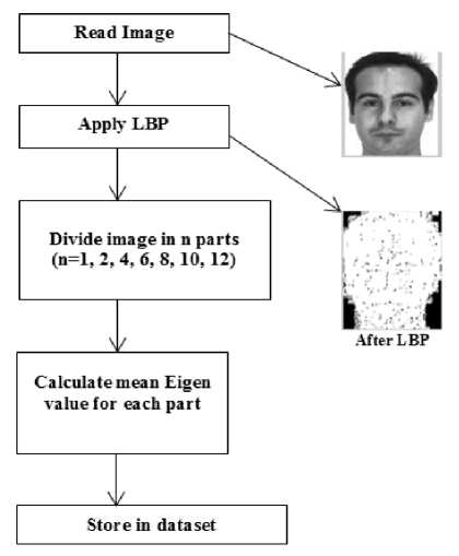
Fig.1. Training phase

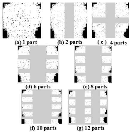
Fig.2. Division of face images into 1, 2, 4, 6, 8, 10 and 12 equal parts after applying LBP

Therefore when the face is taken fully, we get one mean eigen value per face; when the face is divided into two parts, we get two mean eigen values per face. On similar grounds, for n divisions, we get n number of eigen values for the given face.

• B.    Testing phase

The testing phase is similar to the training phase and is shown in Fig. 3. LBP was applied to the image under test and then the image was taken fully in the first case and then in the next cases the image was divided into 2, 4, 6, 8, 10 and 12 equal parts. Then the mean eigen value of each part was computed in the same fashion as that of the training phase. This data is then fed to the SVM classifier which gives any one of the two results: accept or reject.

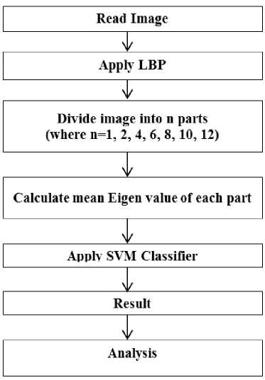
Fig.3. Testing phase.

• IV.    Results and Discussions

This section elaborates each of the 7 cases of feature extraction deployed in the experimentation and the results obtained in this regard.

• Case 1:    No breakdown of images into constituent parts (i.e. full images are taken)

In this case the LBP algorithm was applied to the whole image as shown in Fig. 2 (a) and then applying the PCA algorithm the mean eigen value was taken for each face. Table 1 shows the results obtained for Case 1. In other words, the image was not broken down into any parts, and the whole image was considered for the analysis.

• Case 2:    Dividing the image vertically into 2 equal parts

In this case the LBP algorithm was applied to the whole image and then the image was divided vertically into two equal parts as shown in Fig. 2 (b). And then the PCA algorithm was applied and the mean eigen values were taken for each part. Table 2 shows the results obtained for Case 2. In this case, two feature vectors were obtained.

• Case 3:    Dividing the image into 4 equal parts

In this case the LBP algorithm was applied to the whole image and then the image was divided into four equal parts as shown in Fig. 2 (c) and then applying the PCA algorithm the mean eigen values were taken for each part. Table 3 shows the results obtained for Case 3. Three feature vectors were obtained in this case.

• Case 4:    Dividing the image into 6 equal parts

In this case the LBP algorithm was applied to the whole image and then the image was divided into six equal parts as shown in Fig. 2 (d) and then the PCA algorithm was applied and the mean eigen values were taken for each part. Table 4 shows the results obtained for Case 4. Totally, six feature vectors were obtained in this case.

• Case 5:    Dividing the image into 8 equal parts

In this case the LBP algorithm was applied to the whole image and then the image was divided into eight equal parts as shown in Fig. 2 (e) and then the PCA algorithm was applied and the mean eigen values were taken for each part. Table 5 shows the results obtained for Case 5. Eight feature vectors were obtained in this case.

• Case 6:    Dividing the image into 10 equal parts

In this case the LBP algorithm was applied to the whole image and then the image was divided into ten equal parts as shown in Fig. 2 (f) and then the PCA algorithm was applied and the mean eigen values were taken for each part. Table 6 shows the results obtained for Case 6. Totally 10 feature vectors were obtained in this case.

In case 6, it is observed that when the image was divided into 10 equal parts there was a significant increase in accuracy compared to the previous cases.

• Case 7:    Dividing the image into 12 equal parts

In this case the LBP algorithm was applied to the whole image and then the image was divided into twelve equal parts as shown in Fig. 2 (g) and then the PCA algorithm was applied and the mean eigen values are taken for each part. Table 7 shows the results obtained for Case 7. Totally twelve feature vectors were obtained in this case.

Table 1 through 7 gives the FAR, FRR, accuracy, sensitivity, specificity and execution time for cases 1 through 7, respectively. The numbers of training samples taken from the database were 10, 20, 30 and 40. It was found that FAR was 0% for all the trained sample cases. The parameters like FRR, sensitivity and execution time increased with the size of the database. The accuracy of the algorithm was found to decrease with the increase in the size of the training samples in each of the seven cases.

It was observed in case 7 that when the image is divided into twelve equal parts there was a significant decrease in the accuracy (when compared to case 6); and the optimal accuracy obtained amongst all the cases was in case 6, i.e. when the image was divided into ten equal parts.

Table 1. Accuracy Analysis for 2D face images -one feature with different training sets (Case 1)

Trained Samples	FAR %	FRR %	Accuracy %	Sensitivity	Specificity	Exec Time (ms)
10	0	2	98	0.183673	1	529.688
20	0	10	90	0.333333	1	562.5
30	0	20	80	0.5	1	616.563
40	0	30	70	0.714286	1	671.25

Table 2. Accuracy Analysis for 2D face images - two features with different training sets (Case 2)

Trained Samples	FAR %	FRR %	Accuracy %	Sensitivity	Specificity	Exec Time (ms)
10	0	8	92	0.130435	1	484.063
20	0	14	86	0.302326	1	552.5
30	0	32	68	0.411765	1	585.313
40	0	46	54	0.62963	1	641.25

Table 3. Accuracy Analysis for 2D face images - four features with different training sets (Case 3)

Trained Samples	FAR %	FRR %	Accuracy %	Sensitivity	Specificity	Exec Time (ms)
10	0	4	96	0.166667	1	518.75
20	0	10	90	0.333333	1	578.125
30	0	20	80	0.5	1	640.625
40	0	26	74	0.72973	1	670.625

Table 4. Accuracy Analysis for 2D face images - six features with different training sets (Case 4)

Trained Samples	FAR %	FRR %	Accuracy %	Sensitivity	Specificity	Exec Time (ms)
10	0	4	96	0.166667	1	366.25
20	0	8	92	0.347826	1	412.5
30	0	18	82	0.512195	1	460.625
40	0	22	78	0.74359	1	504.062

Table 5. Accuracy Analysis for 2D face images -eight features with different training sets (case 5)

Trained Samples	FAR %	FRR %	Accuracy %	Sensitivity	Specificity	Exec Time (ms)
10	0	0	100	0.2	NaN	367.5
20	0	6	94	0.361702	1	415.938
30	0	14	86	0.534884	1	460.938
40	0	20	80	0.75	1	590.938

Table 6. Accuracy Analysis for 2D face images - ten features with different training sets (Case 6)

Trained Samples	FAR %	FRR %	Accuracy %	Sensitivity	Specificity	Exec Time (ms)
10	0	0	100	0.2	NaN	355
20	0	0	100	0.4	NaN	401.25
30	0	12	88	0.545455	1	448.438
40	0	18	82	0.756098	1	492.813

Table 7. Accuracy Analysis for 2D face images-twelve features with different training sets (Case 7)

Trained Samples	FAR %	FRR %	Accuracy %	Sensitivity	Specificity	Exec Time (ms)
10	0	2	98	0.183673	1	388.438
20	0	8	92	0.347826	1	444.063
30	0	14	86	0.534884	1	482.188
40	0	18	82	0.756098	1	537.813

Table 8. Accuracy analysis for 2D face images with different features for 50% training (Balanced training)

Number of features	FAR %	FRR %	Accuracy %	Sensitivity	Specificity	Exec Time (ms)
1	0	20	80	0.375	1	594.375
2	0	24	76	0.342105	1	545.313
4	0	18	82	0.390244	1	604.688
6	0	14	86	0.418605	1	429.688
8	0	12	88	0.431818	1	425
10	0	8	92	0.456522	1	427.813
12	0	12	88	0.431818	1	458.438

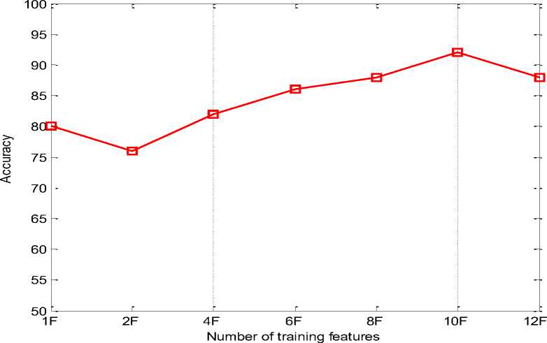
Fig.4. Accuracy comparison for 2D Face recognition for different number of features with 50% training

We further tested the algorithm for balanced training where 25 images were used for training and these images were tested against 50 images of the database for all the cases, wherein the first image was taken whole and then the images were divided into 2, 4, 6, 8, 10 and 12 parts. Balanced training (50% training) is explained in detail in the next section.

• A. Balanced Training

The accuracy for any face recognition algorithm can be correctly interpreted when balanced training is done i.e. half the database is used for training and testing is done against the full database.

In this study, since we have used a database of 50 face images, 25 face images were used for training and they were tested against the 50 face images in the database. The result analysis for balanced training is tabulated in Table 8 for all cases (1, 2, 4, 6, 8, 10 and 12 number of features). Table 8 gives the FAR, FRR, accuracy, sensitivity, specificity and execution time for the proposed methodology for all the cases with ‘n’ number of feature vectors (n = 1, 2, 4, 6, 8, 10 and 12) for 50% training. It was found that the optimal method was Case 6 when the face was divided into ten equal parts where we got the highest accuracy of 92%, FRR of 8%, FAR of 0%, sensitivity of 0.456522, specificity of 1 and execution time of 427.813 milliseconds.

Fig. 4 shows the accuracy analysis for the face images with different number of features (1, 2, 4, 6, 8, 10 and 12) for 50% training. From Fig. 4 it is evident that the face recognition accuracy is highest when the image is divided into ten equal parts. It was also seen that when the image was divided into twelve equal parts the face recognition accuracy decreases. Therefore the optimal method to be used for the proposed algorithm of LBP, PCA and SVM was when the image is divided into ten equal parts.

Fig. 5 gives the summary of the accuracy analysis for different number of features (1 to 12), for 10, 20, 30, 40 and 25 training faces. It was seen that the accuracy was comparatively higher when ten features were extracted from the images.

ROC is used to find an optimal method. The area under the ROC is the measurement of the probability that the distribution of the positive test is statistically larger than the distribution of the negative test. ROC is mainly studied since there is a need to compare different methods applied on the same data, and compare the ROCs to determine which method is the best [17]. Fig. 6 shows the summary of ROC curves for different number of features (1 to 12) for 50% training. When comparing ROC of different tests, good curves lie closer to the top left corner and the worst case is a diagonal line as shown in Fig 6. It was seen that when the ROC curves were plotted for all the cases, the optimal ROC was for the case when ten features were extracted wherein the area under ROC curve is maximum.

Summary of Accuracy Analysis for 2D with SVM

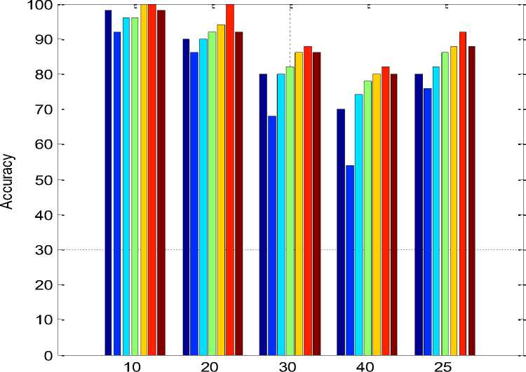
Number of Training Faces

Fig.5. Summary of the accuracy analysis for different number of features and different number of training sets

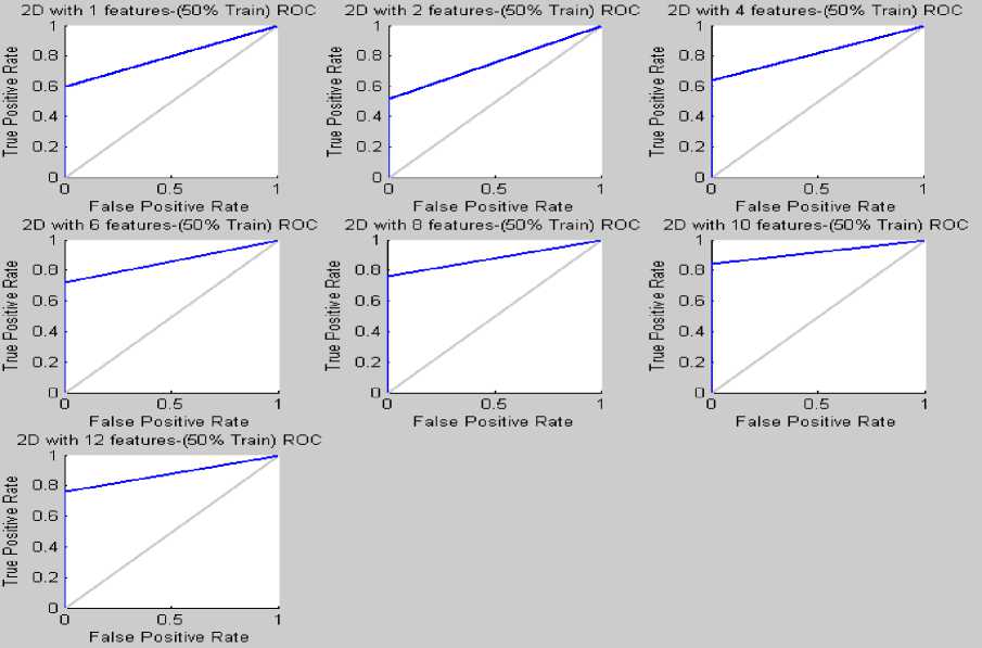
Fig.6. Summary of ROC curves for different number of features (1 to 12) for 50% training

• V. Conclusion

Summarizing the major findings and implications of the proposed method, we found that LBP is fastest execution operator and hence it is most suitable for real time applications. LBP feature vector is used for the removal of illumination problem but it works only on local features and so it cannot capture dominant features with large-scale structures. PCA has high accuracy rate but it has illumination and pose problems. If LBP feature vector is combined with PCA method, it removes the illumination and pose problem and increases recognition rate. Hence this study made use of these two algorithms for feature extraction and SVM was used for classification. The numbers of training samples used were 10, 20, 30, 40 and 25 (balanced training) and the numbers of features used were 1, 2, 4, 6, 8, 10 and 12. It was seen that the accuracy was comparatively higher when 10 features were extracted from the image. Thus the proposed method of recognizing faces worked well on 2D face images. On similar grounds, the study can be extended to 3D face recognition systems.